Single-pixel imaging
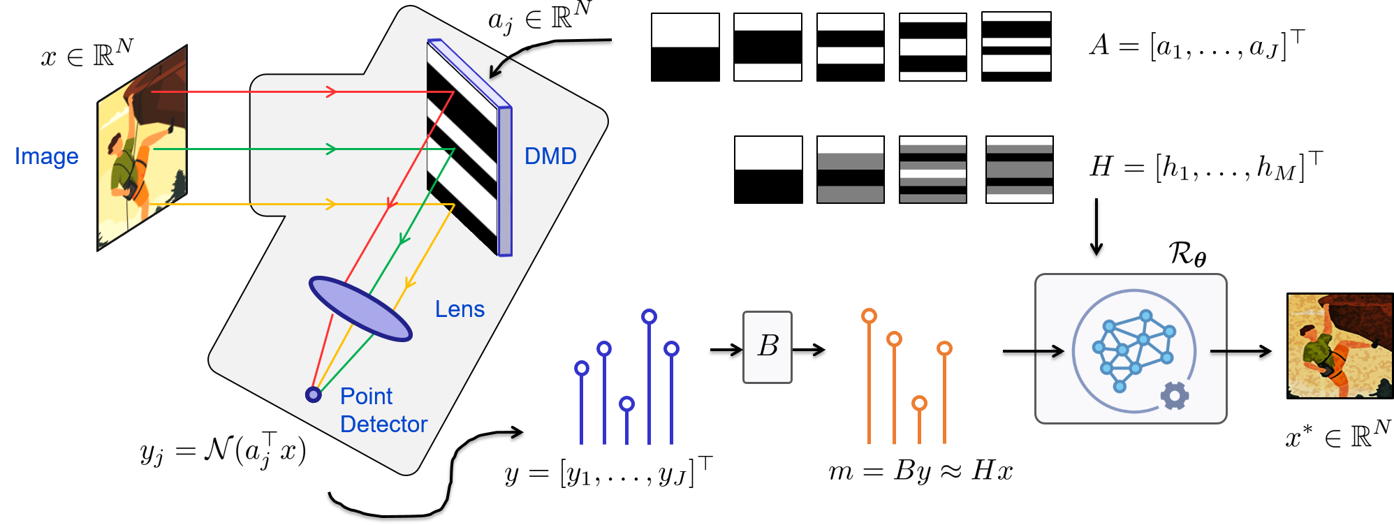
Overview of the principle of single-pixel imaging.
Simulation of the measurements
Single-pixel imaging aims to recover an unknown image \(x\in\mathbb{R}^N\) from a few noisy observations
where \(H\colon \mathbb{R}^{M\times N}\) is a linear measurement operator, \(M\) is the number of measurements and \(N\) is the number of pixels in the image.
In practice, measurements are obtained by uploading a set of light patterns onto a spatial light modulator (e.g., a digital micromirror device (DMD), see principle). Therefore, only positive patterns can be implemented. We model the actual acquisition process as
where \(\mathcal{N} \colon \mathbb{R}^J \to \mathbb{R}^J\) represents a noise operator (e.g., Poisson or Poisson-Gaussian), \(A \in \mathbb{R}_+^{J\times N}\) is the actual acquisition operator that models the (positive) DMD patterns, and \(J\) is the number of DMD patterns.
Handling non negativity with pre-processing
We may preprocess the measurements before reconstruction to transform the actual measurements into the target measurements
where \(B\colon\mathbb{R}^{J}\to \mathbb{R}^{M}\) is the preprocessing operator chosen such that \(BA=H\). Note that the noise of the preprocessed measurements \(m=By\) is not the same as that of the actual measurements \(y\).
Data-driven image reconstruction
Data-driven methods based on deep learning aim to find an estimate \(x^*\in \mathbb{R}^N\) of the unknown image \(x\) from the preprocessed measurements \(By\), using a reconstruction operator \(\mathcal{R}_{\theta^*} \colon \mathbb{R}^M \to \mathbb{R}^N\)
where \(\theta^*\) represents the parameters learned during a training procedure.
Learning phase
In the case of supervised learning, it is assumed that a training dataset \(\{x^{(i)},y^{(i)}\}_{1 \le i \le I}\) of \(I\) pairs of ground truth images in \(\mathbb{R}^N\) and measurements in \(\mathbb{R}^M\) is available}. \(\theta^*\) is then obtained by solving
where \(\mathcal{L}\) is the training loss (e.g., squared error). In the case where only ground truth images \(\{x^{(i)}\}_{1 \le i \le I}\) are available, the associated measurements are simulated as \(y^{(i)} = \mathcal{N}(Ax^{(i)})\), \(1 \le i \le I\).
Reconstruction operator
A simple yet efficient method consists in correcting a traditional (e.g. linear) reconstruction by a data-driven nonlinear step
where \(\mathcal{R}\colon\mathbb{R}^{M}\to\mathbb{R}^N\) is a traditional hand-crafted (e.g., regularized) reconstruction operator and \(\mathcal{G}_\theta\colon\mathbb{R}^{N}\to\mathbb{R}^N\) is a nonlinear neural network that acts in the image domain.
Algorithm unfolding consists in defining \(\mathcal{R}_\theta\) from an iterative scheme
where \(\mathcal{R}_{\theta_k}\) can be interpreted as the computation of the \(k\)-th iteration of the iterative scheme and \(\theta = \bigcup_{k} \theta_k\).