Tutorials
This series of tutorials should guide you through the use of the SPyRiT pipeline.
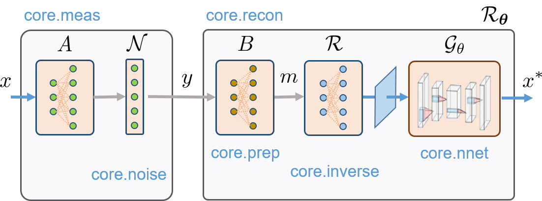
Each tutorial focuses on a specific submodule of the full pipeline.
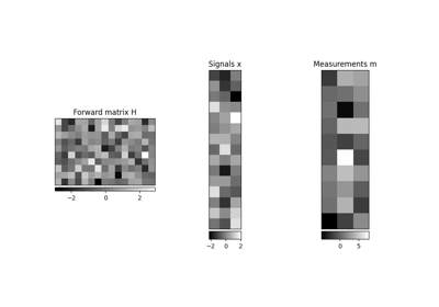
Tutorial 1.a introduces the basics of measurement operators.
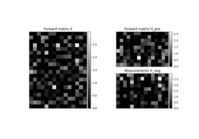
Tutorial 1.b introduces the splitting of measurement operators.
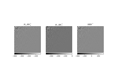
Tutorial 1.c introduces the 2d Hadamard transform with subsampling.
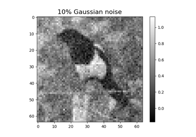
Tutorial 2 introduces the noise operators.
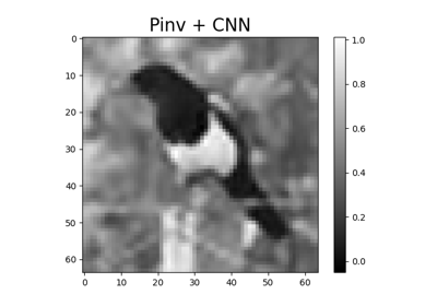
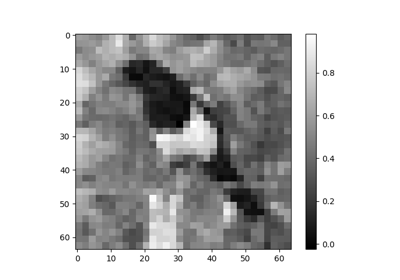
Tutorial 3 demonstrates pseudo-inverse reconstructions from Hadamard measurements.
Tutorial 4.a introduces data-driven post-processing reconstruction.
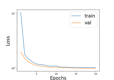
Tutorial 4.b trains the post-processing CNN used in Tutorial 4.a.
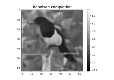
Tutorial 5 introduces the denoised completion network for the reconstruction of Poisson-corrupted subsampled measurements.
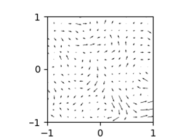
Tutorial 6.a demonstrates how to create and apply deformation fields to simulate motion from static images.
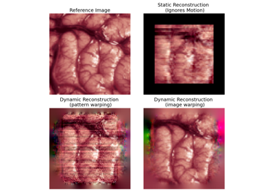
Tutorial 6.b shows how acquire measurements of a moving scene and how to reconstruct a clean image of the scene through motion-compensation.
Note
The Python script (.py) or Jupyter notebook (.ipynb) corresponding to each tutorial can be downloaded at the bottom of the page. The images used in these files can be found on GitHub.
The tutorials below will gradually be updated to be compatible with SPyRiT 3 (work in progress, in the meantime see SPyRiT 2.4.0).
Tutorial 6 uses a Denoised Completion Network with a trainable image denoiser to improve the results obtained in Tutorial 5
Tutorial 7 shows how to perform image reconstruction using a pretrained plug-and-play denoising network.
Tutorial 8 shows how to perform image reconstruction using a learnt proximal gradient descent.
03. Pseudoinverse solution from linear measurements