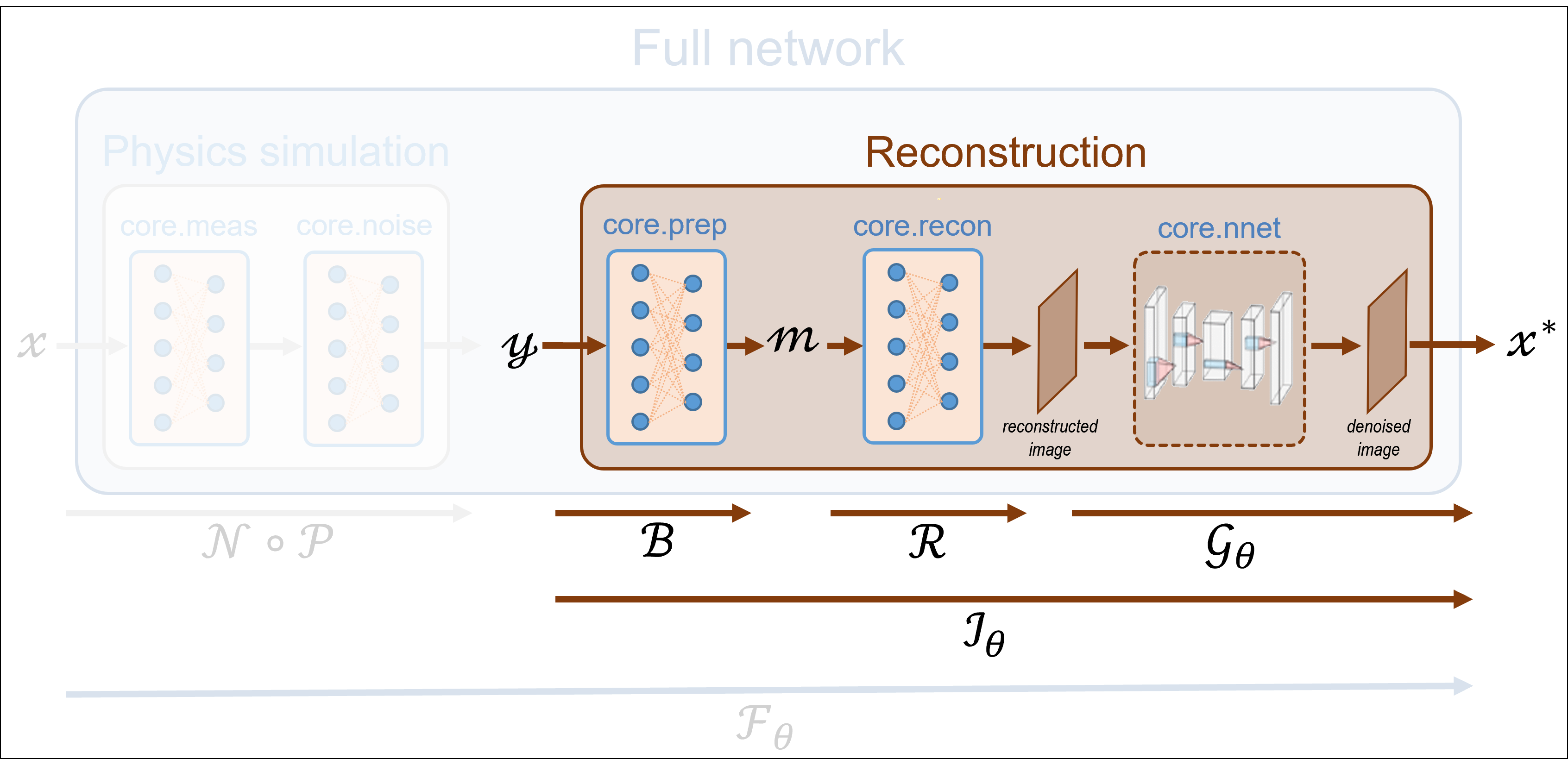
03. Pseudoinverse solution + CNN denoising

This tutorial shows how to simulate measurements and perform image reconstruction using PinvNet (pseudoinverse linear network) with CNN denoising as a last layer. This tutorial is a continuation of the Pseudoinverse solution tutorial but uses a CNN denoiser instead of the identity operator in order to remove artefacts.

The measurement operator is chosen as a Hadamard matrix with positive coefficients, which can be replaced by any matrix.

These tutorials load image samples from /images/.

Load a batch of images

Images \(x\) for training expect values in [-1,1]. The images are normalized using the transform_gray_norm() function.

import os

import torch
import torchvision
import numpy as np
import matplotlib.pyplot as plt

from spyrit.misc.disp import imagesc
from spyrit.misc.statistics import transform_gray_norm

# sphinx_gallery_thumbnail_path = 'fig/tuto3.png'

h = 64  # image size hxh
i = 1  # Image index (modify to change the image)
spyritPath = os.getcwd()
imgs_path = os.path.join(spyritPath, "images/")

# Create a transform for natural images to normalized grayscale image tensors
transform = transform_gray_norm(img_size=h)

# Create dataset and loader (expects class folder 'images/test/')
dataset = torchvision.datasets.ImageFolder(root=imgs_path, transform=transform)
dataloader = torch.utils.data.DataLoader(dataset, batch_size=7)

x, _ = next(iter(dataloader))
print(f"Shape of input images: {x.shape}")

# Select image
x = x[i : i + 1, :, :, :]
x = x.detach().clone()
b, c, h, w = x.shape

# plot
x_plot = x.view(-1, h, h).cpu().numpy()
imagesc(x_plot[0, :, :], r"$x$ in [-1, 1]")

Shape of input images: torch.Size([7, 1, 64, 64])

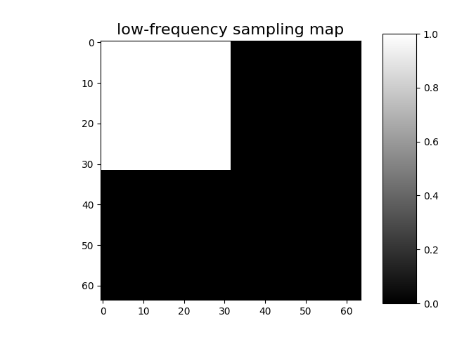
Define a measurement operator

We consider the case where the measurement matrix is the positive component of a Hadamard matrix and the sampling operator preserves only the first M low-frequency coefficients (see Positive Hadamard matrix for full explantion).

import math
from spyrit.misc.sampling import sort_by_significance
from spyrit.misc.walsh_hadamard import walsh2_matrix

F = walsh2_matrix(h)
F = np.where(F > 0, F, 0)
und = 4  # undersampling factor
M = h**2 // und  # number of measurements (undersampling factor = 4)

Sampling_map = np.ones((h, h))
M_xy = math.ceil(M**0.5)
Sampling_map[:, M_xy:] = 0
Sampling_map[M_xy:, :] = 0

F = sort_by_significance(F, Sampling_map, "rows", False)
H = F[:M, :]
print(f"Shape of the measurement matrix: {H.shape}")

imagesc(Sampling_map, "low-frequency sampling map")

Shape of the measurement matrix: (1024, 4096)

Then, we instantiate a spyrit.core.meas.Linear measurement operator

from spyrit.core.meas import Linear

meas_op = Linear(torch.from_numpy(H), pinv=True)

Noiseless case

In the noiseless case, we consider the spyrit.core.noise.NoNoise noise operator

from spyrit.core.noise import NoNoise

N0 = 1.0  # Noise level (noiseless)
noise = NoNoise(meas_op)

# Simulate measurements
y = noise(x.view(b * c, h * w))
print(f"Shape of raw measurements: {y.shape}")

Shape of raw measurements: torch.Size([1, 1024])

We now compute and plot the preprocessed measurements corresponding to an image in [-1,1]

from spyrit.core.prep import DirectPoisson

prep = DirectPoisson(N0, meas_op)  # "Undo" the NoNoise operator

m = prep(y)
print(f"Shape of the preprocessed measurements: {m.shape}")

Shape of the preprocessed measurements: torch.Size([1, 1024])

To display the subsampled measurement vector as an image in the transformed domain, we use the spyrit.misc.sampling.meas2img() function

# plot
from spyrit.misc.sampling import meas2img

m_plot = m.detach().numpy().squeeze()
m_plot = meas2img(m_plot, Sampling_map)
print(f"Shape of the preprocessed measurement image: {m_plot.shape}")

imagesc(m_plot, "Preprocessed measurements (no noise)")

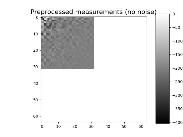
Shape of the preprocessed measurement image: (64, 64)

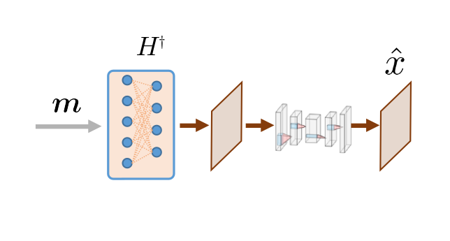
PinvNet Network

We consider the spyrit.core.recon.PinvNet class that reconstructs an image by computing the pseudoinverse solution, which is fed to a neural network denoiser. To compute the pseudoinverse solution only, the denoiser can be set to the identity operator

from spyrit.core.recon import PinvNet

pinv_net = PinvNet(noise, prep, denoi=torch.nn.Identity())

or equivalently

pinv_net = PinvNet(noise, prep)

Then, we reconstruct the image from the measurement vector y using the reconstruct() method

x_rec = pinv_net.reconstruct(y)

Removing artefacts with a CNN

Artefacts can be removed by selecting a neural network denoiser (last layer of PinvNet). We select a simple CNN using the spyrit.core.nnet.ConvNet class, but this can be replaced by any neural network (eg. UNet from spyrit.core.nnet.Unet).

from spyrit.core.nnet import ConvNet, Unet
from spyrit.core.train import load_net

# Define PInvNet with ConvNet denoising layer
denoi = ConvNet()
pinv_net_cnn = PinvNet(noise, prep, denoi)

# Send to GPU if available
device = torch.device("cuda:0" if torch.cuda.is_available() else "cpu")
pinv_net_cnn = pinv_net_cnn.to(device)

As an example, we use a simple ConvNet that has been pretrained using STL-10 dataset. We download the pretrained weights and load them into the network.

# Load pretrained model
model_path = "./model"
num_epochs = 1

pretrained_model_num = 3
if pretrained_model_num == 1:
    # 1 epoch
    url_cnn = "https://drive.google.com/file/d/1iGjxOk06nlB5hSm3caIfx0vy2byQd-ZC/view?usp=drive_link"
    name_cnn = "pinv-net_cnn_stl10_N0_1_N_64_M_1024_epo_1_lr_0.001_sss_10_sdr_0.5_bs_512_reg_1e-07.pth"
    num_epochs = 1
elif pretrained_model_num == 2:
    # 5 epochs
    url_cnn = "https://drive.google.com/file/d/1tzZg1lU3AxOi8-EVXFgnxdtqQCJPjQ9f/view?usp=drive_link"
    name_cnn = (
        "pinv-net_cnn_stl10_N0_1_N_64_M_1024_epo_5_lr_0.001_sss_10_sdr_0.5_bs_512.pth"
    )
    num_epochs = 5
elif pretrained_model_num == 3:
    # 30 epochs
    url_cnn = "https://drive.google.com/file/d/1IZYff1xQxJ3ckAnObqAWyOure6Bjkj4k/view?usp=drive_link"
    name_cnn = "pinv-net_cnn_stl10_N0_1_N_64_M_1024_epo_30_lr_0.001_sss_10_sdr_0.5_bs_512_reg_1e-07.pth"
    num_epochs = 30

# Create model folder
if os.path.exists(model_path) is False:
    os.mkdir(model_path)
    print(f"Created {model_path}")

# Download model weights
model_cnn_path = os.path.join(model_path, name_cnn)
print(model_cnn_path)
if os.path.exists(model_cnn_path) is False:
    try:
        import gdown

        gdown.download(url_cnn, f"{model_cnn_path}.pth", quiet=False, fuzzy=True)
    except:
        print(f"Model {model_cnn_path} not downloaded!")

# Load model weights
load_net(model_cnn_path, pinv_net_cnn, device, False)
print(f"Model {model_cnn_path} loaded.")

Created ./model
./model/pinv-net_cnn_stl10_N0_1_N_64_M_1024_epo_30_lr_0.001_sss_10_sdr_0.5_bs_512_reg_1e-07.pth
Downloading...
From: https://drive.google.com/uc?id=1IZYff1xQxJ3ckAnObqAWyOure6Bjkj4k
To: /home/docs/checkouts/readthedocs.org/user_builds/spyrit/checkouts/2.3.0/tutorial/model/pinv-net_cnn_stl10_N0_1_N_64_M_1024_epo_30_lr_0.001_sss_10_sdr_0.5_bs_512_reg_1e-07.pth.pth

  0%|          | 0.00/50.4M [00:00<?, ?B/s]
 20%|█▉        | 9.96M/50.4M [00:00<00:00, 97.5MB/s]
 60%|██████    | 30.4M/50.4M [00:00<00:00, 158MB/s]
100%|██████████| 50.4M/50.4M [00:00<00:00, 166MB/s]
Model Loaded: ./model/pinv-net_cnn_stl10_N0_1_N_64_M_1024_epo_30_lr_0.001_sss_10_sdr_0.5_bs_512_reg_1e-07.pth
Model ./model/pinv-net_cnn_stl10_N0_1_N_64_M_1024_epo_30_lr_0.001_sss_10_sdr_0.5_bs_512_reg_1e-07.pth loaded.

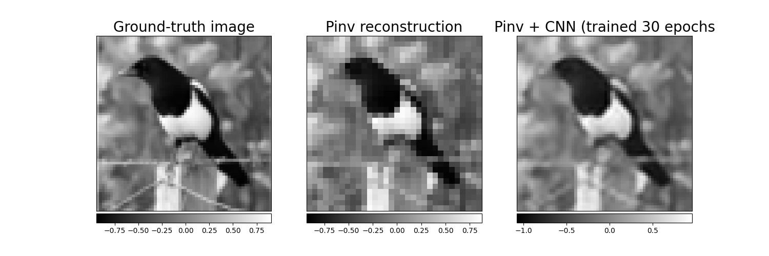
We now reconstruct the image using PinvNet with pretrained CNN denoising and plot results side by side with the PinvNet without denoising

with torch.no_grad():
    x_rec_cnn = pinv_net_cnn.reconstruct(y.to(device))
    x_rec_cnn = pinv_net_cnn(x.to(device))

# plot
x_plot = x.squeeze().cpu().numpy()
x_plot2 = x_rec.squeeze().cpu().numpy()
x_plot3 = x_rec_cnn.squeeze().cpu().numpy()

from spyrit.misc.disp import add_colorbar, noaxis

f, (ax1, ax2, ax3) = plt.subplots(1, 3, figsize=(15, 5))
im1 = ax1.imshow(x_plot, cmap="gray")
ax1.set_title("Ground-truth image", fontsize=20)
noaxis(ax1)
add_colorbar(im1, "bottom", size="20%")

im2 = ax2.imshow(x_plot2, cmap="gray")
ax2.set_title("Pinv reconstruction", fontsize=20)
noaxis(ax2)
add_colorbar(im2, "bottom", size="20%")

im3 = ax3.imshow(x_plot3, cmap="gray")
ax3.set_title(f"Pinv + CNN (trained {num_epochs} epochs", fontsize=20)
noaxis(ax3)
add_colorbar(im3, "bottom", size="20%")

<matplotlib.colorbar.Colorbar object at 0x7ff1e72c7fd0>

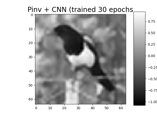
We show the best result again (tutorial thumbnail purpose)

# Plot
imagesc(x_plot3, f"Pinv + CNN (trained {num_epochs} epochs", title_fontsize=20)

plt.show()

In the next tutorial, we will show how to train PinvNet + CNN denoiser.