09. Acquisition and reconstruction of dynamic scenes

This tutorial explains how to reconstruct a motion-compensated image from a dynamic scene.

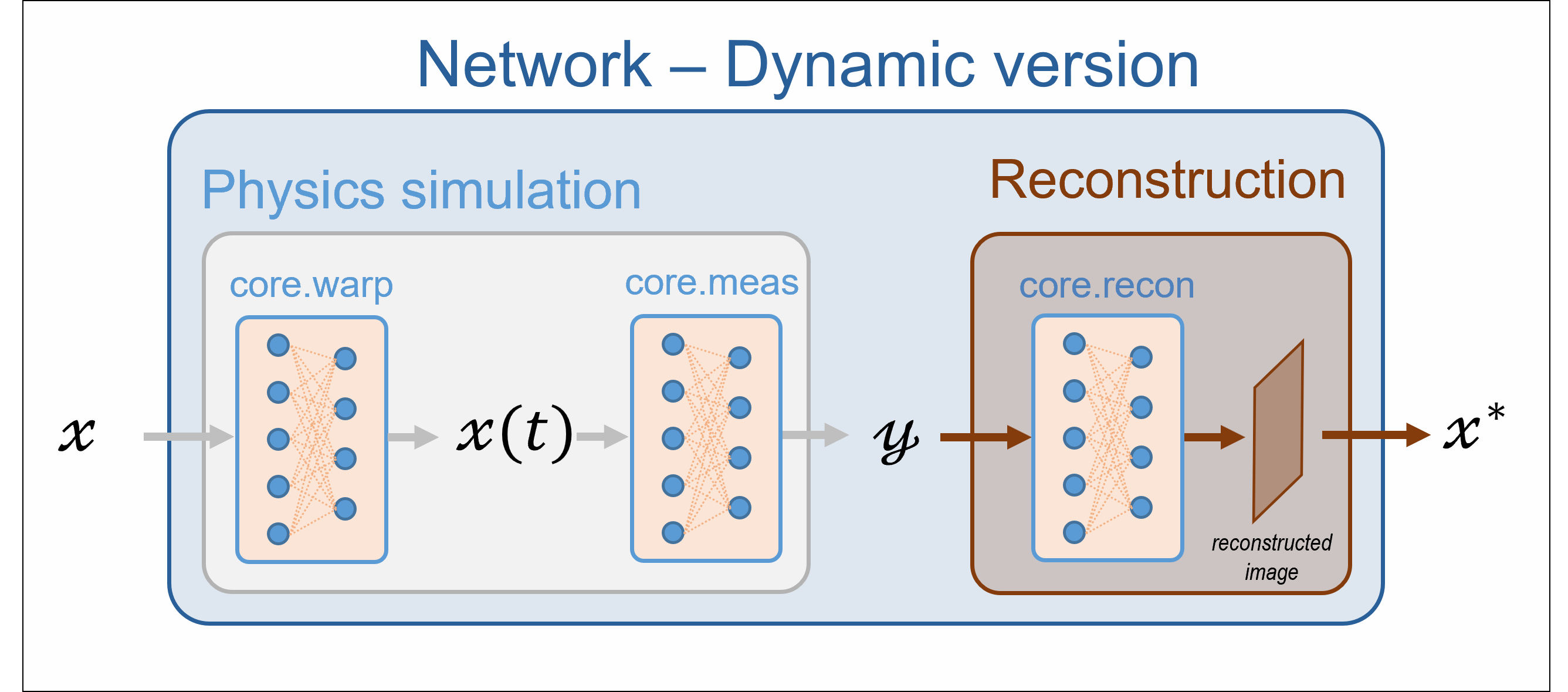
Overview of the dynamic pipeline

There are three steps in the process:

1. Simulation of the dynamic scene. The spyrit.core.warp module can generate multiple frames by warping a static image, given a motion model or deformation field.

2. Simulation of the measurement. The dynamic classes from spyrit.core.meas can simulate the sequence of measurement corresponding to the time frames.

3. Reconstruction of a motion-compensated image from the sequence of measurement.

This tutorial illustrates the three steps through a simple example. Details about the spyrit.core.warp module are included at the end of the example.

1. Generate a video by warping a reference image

Load an image from a batch of images

As in the other tutorials, we load images from the /images/ folder. Here, we consider a 32x32 image for simplicity.

import os

import math
import torch
import torchvision

from spyrit.misc.disp import imagesc
from spyrit.misc.statistics import transform_gray_norm

# sphinx_gallery_thumbnail_path = 'fig/tuto9.png'

img_size = 32  # full image side's size in pixels
meas_size = 32  # measurement pattern side's size in pixels (Hadamard matrix)
img_shape = (img_size, img_size)
meas_shape = (meas_size, meas_size)
i = 1  # Image index (modify to change the image)
spyritPath = os.getcwd()
imgs_path = os.path.join(spyritPath, "images/")


# Create a transform for natural images to normalized grayscale image tensors
transform = transform_gray_norm(img_size=img_size)

# Create dataset and loader (expects class folder 'images/test/')
dataset = torchvision.datasets.ImageFolder(root=imgs_path, transform=transform)
dataloader = torch.utils.data.DataLoader(dataset, batch_size=7)

x, _ = next(iter(dataloader))
print(f"Shape of input images: {x.shape}")

# Select image
x = x[i : i + 1, :, :, :]
x = x.detach().clone()
b, c, h, w = x.shape

# plot
x_plot = x.view(img_shape).cpu()
imagesc(x_plot, r"Original image $x$ in [-1, 1]")

Shape of input images: torch.Size([7, 1, 32, 32])

Define an affine warping

We define an affine transformations using the spyrit.core.warp.AffineDeformationField class, which is instantiated using 3 arguments:

• a function \(f(t)\), where \(t\) represents time,

• a list of times \((t_0, ... , t_n)\) where \(f\) is evaluated,

• the image size (used to determine the grid size) \((height, width)\).

The \(f(t)\) function is a 3x3 matrix-valued function that represents the affine transformation. For more details, see here.

First, we define \(f\) as in [MaBM23] and [MaBP24].

a = 0.2  # amplitude
omega = math.pi  # angular speed


def s(t):
    return 1 + a * math.sin(t * omega)  # base function for f


def f(t):
    return torch.tensor(
        [
            [1 / s(t), 0, 0],
            [0, s(t), 0],
            [0, 0, 1],
        ],
        dtype=torch.float64,
    )

Note

Especially for large images, it is recommended to set the dtype of the output of \(f\) to torch.float64 to reduce numerical errors.

Next, we create the time vector, define the image shape, and compute the deformation field.

from spyrit.core.warp import AffineDeformationField

time_vector = torch.linspace(0, 10, (meas_size**2) * 2)  # *2 because of the splitting
aff_field = AffineDeformationField(f, time_vector, img_shape)

Note

The number of measurement patterns must match the number of frames of the video. Therefore, we set the number of frames to the square of the measurement size.

Warp the image

Warping works with vectorized images. So, we first reshape the image from (b,c,h,w) to (c, h*w)

x = x.view(c, h * w)

We can now warp the image

x_motion = aff_field(x, 0, (meas_size**2) * 2)
c, n_frames, n_pixels = x_motion.shape

Note

Currently, the AffineDeformationField and DeformationField can only warp a single image at a time.

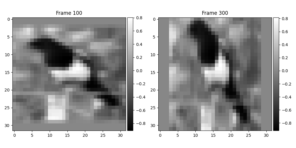
Plot two time frames

import matplotlib.pyplot as plt
from spyrit.misc.disp import add_colorbar

frames = [100, 300]

plot, axes = plt.subplots(1, len(frames), figsize=(10, 5))

for i, f in enumerate(frames):
    im = axes[i].imshow(x_motion[0, f, :].view(img_shape).cpu().numpy(), cmap="gray")
    axes[i].set_title(f"Frame {f}")
    add_colorbar(im, "right", size="20%")
plot.tight_layout()
plt.show()

2. Simulation of the measurements

In this section, we simulate the acquisition of the previous video. We consider a full Hadamard matrix (no subsampling) using the spyrit.core.meas.DynamicHadamSplit class.

Note

For the moment, no noise can be applied to the dynamic measurement operators. This will be available in a future release. As a consequence, the preprocessing operators are also unavailable.

Instantiation of a dynamic measurement operator

The DynamicHadamSplit class is the counterpart of the HadamardSplit class for dynamic scenes. The dynamic measurement operator considers a different frame for each of the measurement patterns. Therefore, the number of frames in the video must be the same as the number of measurement patterns .

from spyrit.core.meas import DynamicHadamSplit

meas_op = DynamicHadamSplit(M=meas_size**2, h=meas_size, Ord=None, img_shape=img_shape)

# show the measurement matrix H
print("Shape of the measurement matrix H:", meas_op.H_static.shape)
# as we are using split measurements, it is the matrix P that is effectively
# used when computing the measurements
print("Shape of the measurement matrix P:", meas_op.P.shape)

Shape of the measurement matrix H: torch.Size([1024, 1024])
Shape of the measurement matrix P: torch.Size([2048, 1024])

Note

If there are too many frames in your video, you may want to use only the first frames of it. If there are too many patterns in your acquisition operator, you may want to reduce this number by setting the parameter M.

Simulation

As in the static case, this is done by calling (implicitly) forward method.

y = meas_op(x_motion)

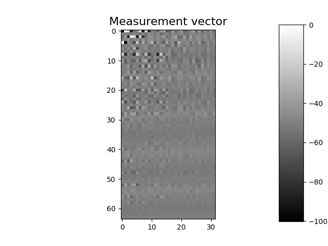
Plot the measurements

imagesc(y.view((meas_size * 2, meas_size)).cpu().numpy(), "Measurement vector")

3. Reconstruction of the motion-compensated (reference) image

In this section, we reconstruct the motion-compensated (reference) image from the dynamic measurements. This a two-step approach:

1. Construction of a dynamic forward matrix that combines the knowledge of the measurement patterns and the deformation field.

2. Resolution of a linear problem based on the dynamic forward matrix.

For details, refer to [MaBM23] and [MaBP24].

Computation of the dynamic measurement matrix

The dynamic measurement matrix \(H_{\rm dyn}\) is defined as the measurement matrix that gives the dynamic measurement vector \(y\) from the reference image \(x_{\rm ref}\)

\[y = H_{\rm dyn} x_{\rm ref}\]

The dynamic measurement matrix is built by calling the build_H_dyn() method of the measurement operator, given a deformation field.

print("H_dyn computed:", hasattr(meas_op, "H_dyn"))

meas_op.build_H_dyn(aff_field, mode="bilinear")
print("H_dyn computed:", hasattr(meas_op, "H_dyn"))

H_dyn computed: False
H_dyn computed: True

This method adds to the measurement operator a new attribute named H_dyn. It can also be accessed using the attribute name H for compatibility reasons, although it is NOT recommended.

Note

There are different strategies for building \(H_{\rm dyn}\). Here, we consider the method described in [MaBP24] that avoids warping the Hadamard patterns.

Note

Here, the deformation field is known. In the general case, it will have to be estimated.

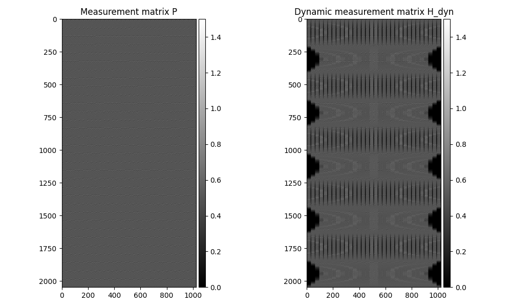
Important

The dynamic measurement matrix H_dyn is computed from the actual measurement matrix \(P\) that is obtained by splitting the Hadamard matrix (see Tutorial 5). This can be seen by checking their shapes, which are the transpose of each other.

# recommended way
print("H_dyn shape:", meas_op.H_dyn.shape)
print("P shape:", meas_op.P.shape)
# NOT recommended, can cause confusions
print("H shape:", meas_op.H.shape)
print("H_dyn is same as H:", (meas_op.H == meas_op.H_dyn).all())

H_dyn shape: torch.Size([2048, 1024])
P shape: torch.Size([2048, 1024])
H shape: torch.Size([2048, 1024])
H_dyn is same as H: tensor(True)

We plot the actual and dynamic measurement matrix

plot, (ax1, ax2) = plt.subplots(1, 2, figsize=(10, 6))

im1 = ax1.imshow(meas_op.P.cpu().numpy(), vmin=0, vmax=1.5, cmap="gray")
ax1.set_title("Measurement matrix P")
add_colorbar(im1, "right", size="20%")

im2 = ax2.imshow(meas_op.H_dyn.cpu().numpy(), vmin=0, vmax=1.5, cmap="gray")
ax2.set_title("Dynamic measurement matrix H_dyn")
add_colorbar(im2, "right", size="20%")

plot.tight_layout()
plt.show()

Reconstruction

We first compute the pseudo-inverse of the dynamic measurement matrix by calling the build_H_dyn_pinv() method that allows regularization.

print("H_dyn_pinv computed:", hasattr(meas_op, "H_dyn_pinv"))
meas_op.build_H_dyn_pinv(reg="L2", eta=1e-6)
print("H_dyn_pinv computed:", hasattr(meas_op, "H_dyn_pinv"))

H_dyn_pinv computed: False
H_dyn_pinv computed: True

This creates a new attribute H_dyn_pinv that stores the pseudo-inverse of H_dyn. As before, the same tensor can be accessed through the attribute H_pinv, for compatibility reasons, although it is not recommended.

Next, we simply call the pinv() method.

x_hat1 = meas_op.pinv(y)
print("x_hat1 shape:", x_hat1.shape)

x_hat1 shape: torch.Size([1, 1024])

As in the static case, this can also be done through using spyrit.core.recon.PseudoInverse class.

from spyrit.core.recon import PseudoInverse

recon_op = PseudoInverse()
x_hat2 = recon_op(y, meas_op)

print("x_hat1 and x_hat2 are equal:", (x_hat1 == x_hat2).all())

x_hat1 and x_hat2 are equal: tensor(True)

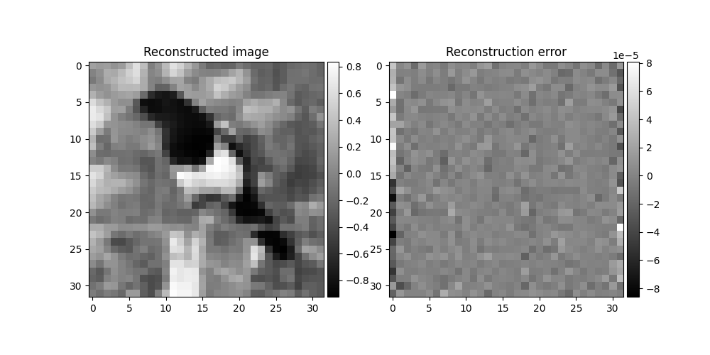
We finally plot the reconstructed image and its difference with the ground-truth image

plot, (ax1, ax2) = plt.subplots(1, 2, figsize=(10, 5))

im1 = ax1.imshow(x_hat1.view(img_shape), cmap="gray")
ax1.set_title("Reconstructed image")
add_colorbar(im1, "right", size="20%")

im2 = ax2.imshow(x_plot.view(img_shape) - x_hat1.view(img_shape), cmap="gray")
ax2.set_title("Reconstruction error")
add_colorbar(im2, "right", size="20%")

# plot.tight_layout()
plt.show()

Note

As with static reconstruction, it is possible to reconstruct the motion-compensated image without having to compute the pseudo-inverse explicitly. Calling the method pinv() while the attribute H_dyn_pinv is not defined will result in using the torch.linalg.lstsq() solver.

4. Warping detailed explanation

This tutorial uses the class spyrit.core.warp.AffineDeformationField to simulate the movement of a still image. This class is a subclass of spyrit.core.warp.DeformationField, which can be used to deform an image in a more general manner. This is particularly useful for experimental setups where the deformation is estimated from real measurements.

Here, we provide an example of how to use the class spyrit.core.warp.DeformationField. The class takes one argument: the deformation field itself of shape \((n_{\rm frames},h,w,2)\), where \(n_{\rm frames}\) is the number of frames, and \(h\) and \(w\) are the height and width of the image. The last dimension represents the 2D pixel from where to interpolate the new pixel value at the coordinate \((h,w)\).

We will first use an instance of spyrit.core.warp.AffineDeformationField to create the deformation field. Then, a separate instance of spyrit.core.warp.DeformationField will be created using the deformation field from the affine deformation field.

from spyrit.core.warp import DeformationField

# define a rotation function
omega = 2 * math.pi  # angular velocity


def rot(t):
    ans = torch.tensor(
        [
            [math.cos(t * omega), -math.sin(t * omega), 0],
            [math.sin(t * omega), math.cos(t * omega), 0],
            [0, 0, 1],
        ],
        dtype=torch.float64,
    )  # it is recommended to use float64
    return ans


# create a time vector of length 100 (change this to fit your needs)
t0 = 0
t1 = 10
n_frames = 100
time_vector = torch.linspace(t0, t1, n_frames)
img_shape = (50, 50)  # image shape

# create the affine deformation field
aff_field2 = AffineDeformationField(rot, time_vector, img_shape)

Now that the affine deformation field is created, we can access the deformation field through the attribute field. Its value can then be used to create a new instance of spyrit.core.warp.DeformationField.

# get the deformation field
field = aff_field2.field
print("field shape:", field.shape)

# create an instance of DeformationField
def_field = DeformationField(field)

# def_field and aff_field2 are the same
print("def_field and aff_field2 are the same:", (def_field == aff_field2))

field shape: torch.Size([100, 50, 50, 2])
def_field and aff_field2 are the same: True

References for dynamic reconstruction

[MaBM23] (1,2)

Thomas Maitre, Elie Bretin, L. Mahieu-Williame, Michaël Sdika, Nicolas Ducros. Hybrid single-pixel camera for dynamic hyperspectral imaging. 2023. hal-04310110

[MaBP24] (1,2,3)

(MICCAI 2024 paper #1903) Thomas Maitre, Elie Bretin, Romain Phan, Nicolas Ducros, Michaël Sdika. Dynamic Single-Pixel Imaging on an Extended Field of View without Warping the Patterns. 2024. hal-04533981