06. Denoised Completion Network (DCNet)

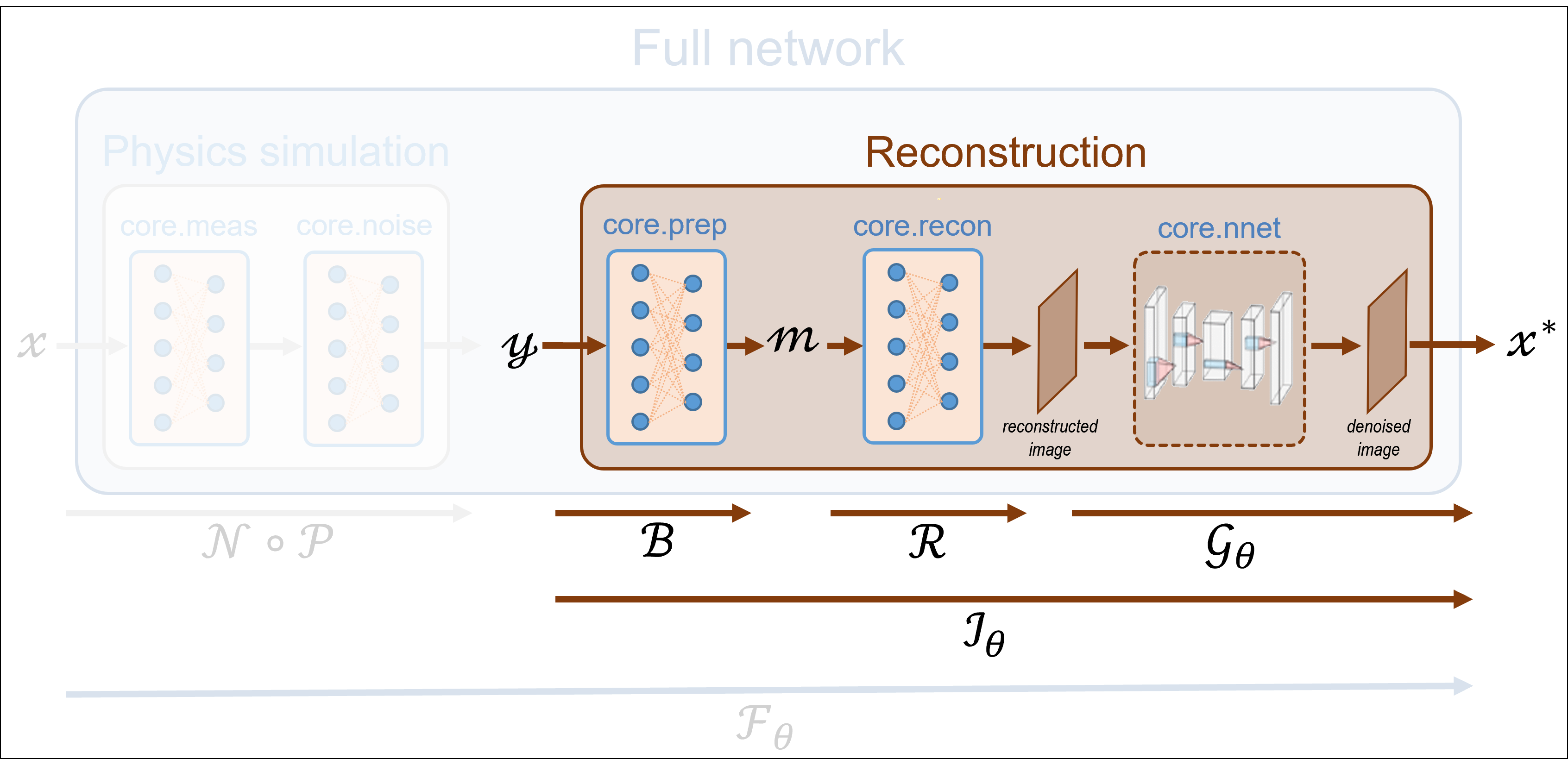
This tutorial shows how to perform image reconstruction using the denoised completion network (DCNet) with a trainable image denoiser. In the next tutorial, we will plug a denoiser into a DCNet, which requires no training.

Note

As in the previous tutorials, we consider a split Hadamard operator and measurements corrupted by Poisson noise (see Tutorial 5).

Load a batch of images

Update search path

# sphinx_gallery_thumbnail_path = 'fig/tuto6.png'
import os

spyritPath = os.getcwd()
imgs_path = os.path.join(spyritPath, "images/")

Images \(x\) for training neural networks expect values in [-1,1]. The images are normalized and resized using the transform_gray_norm() function.

from spyrit.misc.statistics import transform_gray_norm

h = 64  # image is resized to h x h
transform = transform_gray_norm(img_size=h)

Create a data loader from some dataset (images must be in the folder images/test/)

import torch
import torchvision

dataset = torchvision.datasets.ImageFolder(root=imgs_path, transform=transform)
dataloader = torch.utils.data.DataLoader(dataset, batch_size=7)

x, _ = next(iter(dataloader))
print(f"Shape of input images: {x.shape}")

Shape of input images: torch.Size([7, 1, 64, 64])

Select the i-th image in the batch

i = 1  # Image index (modify to change the image)
x = x[i : i + 1, :, :, :]
x = x.detach().clone()
b, c, h, w = x.shape

Plot the selected image

from spyrit.misc.disp import imagesc

x_plot = x.view(-1, h, h).cpu().numpy()
imagesc(x_plot[0, :, :], r"$x$ in [-1, 1]")

Forward operators for split measurements

We consider noisy measurements obtained from a split Hadamard operator, and a subsampling strategy that retaines the coefficients with the largest variance (for more details, refer to Tutorial 5).

First, we download the covariance matrix from our warehouse.

import girder_client
import numpy as np

# api Rest url of the warehouse
url = "https://pilot-warehouse.creatis.insa-lyon.fr/api/v1"
# Generate the warehouse client
gc = girder_client.GirderClient(apiUrl=url)
# Download the covariance matrix and mean image
data_folder = "./stat/"
dataId_list = [
    "63935b624d15dd536f0484a5",  # for reconstruction (imageNet, 64)
    "63935a224d15dd536f048496",  # for reconstruction (imageNet, 64)
]
cov_name = "./stat/Cov_64x64.npy"
try:
    Cov = np.load(cov_name)
    print(f"Cov matrix {cov_name} loaded")
except FileNotFoundError:
    for dataId in dataId_list:
        myfile = gc.getFile(dataId)
        gc.downloadFile(dataId, data_folder + myfile["name"])
    print(f"Created {data_folder}")
    Cov = np.load(cov_name)
    print(f"Cov matrix {cov_name} loaded")
except:
    Cov = np.eye(h * h)
    print(f"Cov matrix {cov_name} not found! Set to the identity")

Cov matrix ./stat/Cov_64x64.npy loaded

We define the measurement, noise and preprocessing operators and then simulate a measurement vector corrupted by Poisson noise. As in the previous tutorials, we simulate an accelerated acquisition by subsampling the measurement matrix by retaining only the first rows of a Hadamard matrix that is permuted looking at the diagonal of the covariance matrix.

from spyrit.core.meas import HadamSplit
from spyrit.core.noise import Poisson
from spyrit.misc.sampling import meas2img
from spyrit.misc.statistics import Cov2Var
from spyrit.core.prep import SplitPoisson

# Measurement parameters
M = 64 * 64 // 4  # Number of measurements (here, 1/4 of the pixels)
alpha = 100.0  # number of photons

# Measurement and noise operators
Ord = Cov2Var(Cov)
meas_op = HadamSplit(M, h, torch.from_numpy(Ord))
noise_op = Poisson(meas_op, alpha)
prep_op = SplitPoisson(alpha, meas_op)

# Vectorize image
x = x.view(b * c, h * w)
print(f"Shape of vectorized image: {x.shape}")
# Measurements
y = noise_op(x)  # a noisy measurement vector
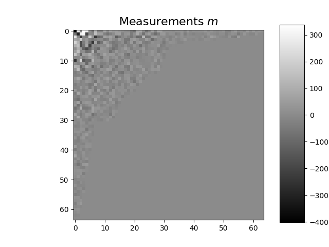
m = prep_op(y)  # preprocessed measurement vector

m_plot = m.detach().numpy()
m_plot = meas2img(m_plot, Ord)
imagesc(m_plot[0, :, :], r"Measurements $m$")

Shape of vectorized image: torch.Size([1, 4096])

Pseudo inverse solution

We compute the pseudo inverse solution using spyrit.core.recon.PinvNet class as in the previous tutorial.

# Instantiate a PinvNet (with no denoising by default)
from spyrit.core.recon import PinvNet

pinvnet = PinvNet(noise_op, prep_op)

# Use GPU, if available
device = torch.device("cuda:0" if torch.cuda.is_available() else "cpu")
pinvnet = pinvnet.to(device)
y = y.to(device)

# Reconstruction
with torch.no_grad():
    z_invnet = pinvnet.reconstruct(y)

Denoised completion network (DCNet)

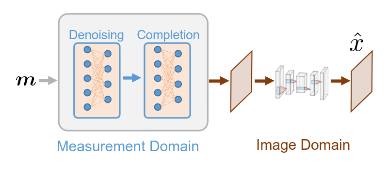
The DCNet is based on four sequential steps:

1. Denoising in the measurement domain.

2. Estimation of the missing measurements from the denoised ones.

3. Image-domain mapping.

4. (Learned) Denoising in the image domain.

Typically, only the last step involves learnable parameters.

Denoised completion

The first three steps implement denoised completion, which corresponds to Tikhonov regularization. Considering linear measurements \(y = Hx\), where \(H\) is the measurement matrix and \(x\) is the unknown image, it estimates \(x\) from \(y\) by minimizing

\[\| y - Hx \|^2_{\Sigma^{-1}_\alpha} + \|x\|^2_{\Sigma^{-1}},\]

where \(\Sigma\) is a covariance prior and \(\Sigma_\alpha\) is the noise covariance. Denoised completation can be performed using the TikhonovMeasurementPriorDiag class (see documentation for more details).

In practice, it is more convenient to use the spyrit.core.recon.DCNet class, which relies on a forward operator, a preprocessing operator, and a covariance prior.

from spyrit.core.recon import DCNet

dcnet = DCNet(noise_op, prep_op, torch.from_numpy(Cov))

# Use GPU, if available
dcnet = dcnet.to(device)
y = y.to(device)

with torch.no_grad():
    z_dcnet = dcnet.reconstruct(y)

Note

In this tutorial, the covariance matrix used to define subsampling is also used as prior knowledge during reconstruction.

(Learned) Denoising in the image domain

To implement denoising in the image domain, we provide a spyrit.core.nnet.Unet denoiser to a spyrit.core.recon.DCNet.

from spyrit.core.nnet import Unet

denoi = Unet()
dcnet_unet = DCNet(noise_op, prep_op, torch.from_numpy(Cov), denoi)
dcnet_unet = dcnet_unet.to(device)  # Use GPU, if available

We load pretrained weights for the UNet

from spyrit.core.train import load_net

# Download weights
url_unet = "https://drive.google.com/file/d/15PRRZj5OxKpn1iJw78lGwUUBtTbFco1l/view?usp=drive_link"
model_path = "./model"
if os.path.exists(model_path) is False:
    os.mkdir(model_path)
    print(f"Created {model_path}")
model_unet_path = os.path.join(
    model_path,
    "dc-net_unet_stl10_N0_100_N_64_M_1024_epo_30_lr_0.001_sss_10_sdr_0.5_bs_512_reg_1e-07.pth",
)
load_unet = True
if os.path.exists(model_unet_path) is False:
    try:
        import gdown

        gdown.download(url_unet, f"{model_unet_path}.pth", quiet=False, fuzzy=True)
    except:
        print(f"Model {model_unet_path} not found!")
        load_unet = False
if load_unet:
    # Load pretrained model
    load_net(model_unet_path, dcnet_unet, device, False)
    # print(f"Model {model_unet_path} loaded.")

Downloading...
From: https://drive.google.com/uc?id=15PRRZj5OxKpn1iJw78lGwUUBtTbFco1l
To: /home/docs/checkouts/readthedocs.org/user_builds/spyrit/checkouts/2.3.0/tutorial/model/dc-net_unet_stl10_N0_100_N_64_M_1024_epo_30_lr_0.001_sss_10_sdr_0.5_bs_512_reg_1e-07.pth.pth

  0%|          | 0.00/149M [00:00<?, ?B/s]
  3%|▎         | 4.72M/149M [00:00<00:04, 30.1MB/s]
 12%|█▏        | 17.3M/149M [00:00<00:02, 60.1MB/s]
 17%|█▋        | 25.7M/149M [00:00<00:02, 56.6MB/s]
 23%|██▎       | 34.1M/149M [00:00<00:01, 61.5MB/s]
 29%|██▊       | 42.5M/149M [00:00<00:01, 63.5MB/s]
 34%|███▍      | 50.9M/149M [00:00<00:01, 65.3MB/s]
 40%|███▉      | 59.2M/149M [00:00<00:01, 65.9MB/s]
 45%|████▌     | 67.6M/149M [00:01<00:01, 66.7MB/s]
 57%|█████▋    | 84.4M/149M [00:01<00:00, 84.1MB/s]
 68%|██████▊   | 101M/149M [00:01<00:00, 94.8MB/s]
 79%|███████▉  | 118M/149M [00:01<00:00, 104MB/s]
 91%|█████████ | 135M/149M [00:01<00:00, 82.8MB/s]
100%|██████████| 149M/149M [00:01<00:00, 79.7MB/s]
Model Loaded: ./model/dc-net_unet_stl10_N0_100_N_64_M_1024_epo_30_lr_0.001_sss_10_sdr_0.5_bs_512_reg_1e-07.pth

We reconstruct the image

with torch.no_grad():
    z_dcnet_unet = dcnet_unet.reconstruct(y)

Results

import matplotlib.pyplot as plt
from spyrit.misc.disp import add_colorbar, noaxis

x_plot = x.view(-1, h, h).cpu().numpy()
x_plot2 = z_invnet.view(-1, h, h).cpu().numpy()
x_plot3 = z_dcnet.view(-1, h, h).cpu().numpy()
x_plot4 = z_dcnet_unet.view(-1, h, h).cpu().numpy()
f, axs = plt.subplots(2, 2, figsize=(10, 10))

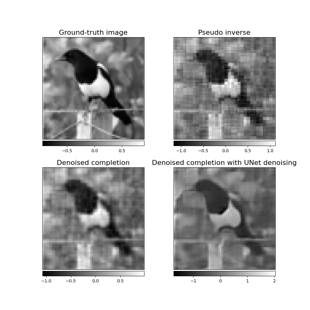
# Plot the ground-truth image
im1 = axs[0, 0].imshow(x_plot[0, :, :], cmap="gray")
axs[0, 0].set_title("Ground-truth image", fontsize=16)
noaxis(axs[0, 0])
add_colorbar(im1, "bottom")

# Plot the pseudo inverse solution
im2 = axs[0, 1].imshow(x_plot2[0, :, :], cmap="gray")
axs[0, 1].set_title("Pseudo inverse", fontsize=16)
noaxis(axs[0, 1])
add_colorbar(im2, "bottom")

# Plot the solution obtained from denoised completion
im3 = axs[1, 0].imshow(x_plot3[0, :, :], cmap="gray")
axs[1, 0].set_title(f"Denoised completion", fontsize=16)
noaxis(axs[1, 0])
add_colorbar(im3, "bottom")

# Plot the solution obtained from denoised completion with UNet denoising
im4 = axs[1, 1].imshow(x_plot4[0, :, :], cmap="gray")
axs[1, 1].set_title(f"Denoised completion with UNet denoising", fontsize=16)
noaxis(axs[1, 1])
add_colorbar(im4, "bottom")

plt.show()

Note

While the pseudo inverse reconstrcution is pixelized, the solution obtained by denoised completion is smoother. DCNet with UNet denoising in the image domain provides the best reconstruction.

Note

We refer to spyrit-examples tutorials for a comparison of different solutions (pinvNet, DCNet and DRUNet) that can be run in colab.