04. Train pseudoinverse solution + CNN denoising

This tutorial shows how to train PinvNet with a CNN denoiser for reconstruction of linear measurements (results shown in the previous tutorial). As an example, we use a small CNN, which can be replaced by any other network, for example Unet. Training is performed on the STL-10 dataset.

You can use Tensorboard for Pytorch for experiment tracking and for visualizing the training process: losses, network weights, and intermediate results (reconstructed images at different epochs).

The linear measurement operator is chosen as the positive part of a Hadamard matrix, but this matrix can be replaced by any desired matrix.

These tutorials load image samples from /images/.

Load a batch of images

First, we load an image \(x\) and normalized it to [-1,1], as in previous examples.

import os

import torch
import torchvision
import matplotlib.pyplot as plt

import spyrit.core.torch as spytorch
from spyrit.misc.disp import imagesc
from spyrit.misc.statistics import transform_gray_norm

h = 64  # image size hxh
i = 1  # Image index (modify to change the image)
spyritPath = os.getcwd()
imgs_path = os.path.join(spyritPath, "images/")


# Create a transform for natural images to normalized grayscale image tensors
transform = transform_gray_norm(img_size=h)

# Create dataset and loader (expects class folder 'images/test/')
dataset = torchvision.datasets.ImageFolder(root=imgs_path, transform=transform)
dataloader = torch.utils.data.DataLoader(dataset, batch_size=7)

x, _ = next(iter(dataloader))
print(f"Shape of input images: {x.shape}")

# Select image
x = x[i : i + 1, :, :, :]
x = x.detach().clone()
print(f"Shape of selected image: {x.shape}")
b, c, h, w = x.shape

# plot
imagesc(x[0, 0, :, :], r"$x$ in [-1, 1]")

Shape of input images: torch.Size([7, 1, 64, 64])
Shape of selected image: torch.Size([1, 1, 64, 64])
/home/docs/checkouts/readthedocs.org/user_builds/spyrit/envs/2.4.0/lib/python3.11/site-packages/matplotlib/cbook.py:684: DeprecationWarning: __array__ implementation doesn't accept a copy keyword, so passing copy=False failed. __array__ must implement 'dtype' and 'copy' keyword arguments. To learn more, see the migration guide https://numpy.org/devdocs/numpy_2_0_migration_guide.html#adapting-to-changes-in-the-copy-keyword
  x = np.array(x, subok=True, copy=copy)

Define a dataloader

We define a dataloader for STL-10 dataset using spyrit.misc.statistics.data_loaders_stl10(). This will download the dataset to the provided path if it is not already downloaded. It is based on pytorch pre-loaded dataset torchvision.datasets.STL10 and torch.utils.data.DataLoader, which creates a generator that iterates through the dataset, returning a batch of images and labels at each iteration.

Set mode_run to True in the script below to download the dataset and for training; otherwise, pretrained weights and results will be download for display.

from spyrit.misc.statistics import data_loaders_stl10
from pathlib import Path

# Parameters
h = 64  # image size hxh
data_root = Path("./data")  # path to data folder (where the dataset is stored)
batch_size = 512

# Dataloader for STL-10 dataset
mode_run = False
if mode_run:
    dataloaders = data_loaders_stl10(
        data_root,
        img_size=h,
        batch_size=batch_size,
        seed=7,
        shuffle=True,
        download=True,
    )

Define a measurement operator

We consider the case where the measurement matrix is the positive component of a Hadamard matrix, which is often used in single-pixel imaging (see Hadamard matrix). Then, we simulate an accelerated acquisition by keeping only the first M low-frequency coefficients (see low frequency sampling).

import math

und = 4  # undersampling factor
M = h**2 // und  # number of measurements (undersampling factor = 4)

F = spytorch.walsh2_matrix(h)
F = torch.max(F, torch.zeros_like(F))

Sampling_map = torch.zeros(h, h)
M_xy = math.ceil(M**0.5)
Sampling_map[:M_xy, :M_xy] = 1

# imagesc(Sampling_map, 'low-frequency sampling map')

F = spytorch.sort_by_significance(F, Sampling_map, "rows", False)
H = F[:M, :]

print(f"Shape of the measurement matrix: {H.shape}")

Shape of the measurement matrix: torch.Size([1024, 4096])

Then, we instantiate a spyrit.core.meas.Linear measurement operator, a spyrit.core.noise.NoNoise noise operator for noiseless case, and a preprocessing measurements operator spyrit.core.prep.DirectPoisson.

from spyrit.core.meas import Linear
from spyrit.core.noise import NoNoise
from spyrit.core.prep import DirectPoisson

meas_op = Linear(H, pinv=True)
noise = NoNoise(meas_op)
N0 = 1.0  # Mean maximum total number of photons
prep = DirectPoisson(N0, meas_op)  # "Undo" the NoNoise operator

PinvNet Network

We consider the spyrit.core.recon.PinvNet class that reconstructs an image by computing the pseudoinverse solution and applies a nonlinear network denoiser. First, we must define the denoiser. As an example, we choose a small CNN using the spyrit.core.nnet.ConvNet class. Then, we define the PinvNet network by passing the noise and preprocessing operators and the denoiser.

from spyrit.core.nnet import ConvNet
from spyrit.core.recon import PinvNet

denoiser = ConvNet()
model = PinvNet(noise, prep, denoi=denoiser)

# Send to GPU if available
device = torch.device("cuda:0" if torch.cuda.is_available() else "cpu")

# Use multiple GPUs if available
if torch.cuda.device_count() > 1:
    print("Let's use", torch.cuda.device_count(), "GPUs!")
    model = nn.DataParallel(model)

print("Using device:", device)
model = model.to(device)

Using device: cpu

Note

In the example provided, we choose a small CNN using the spyrit.core.nnet.ConvNet class. This can be replaced by any denoiser, for example the spyrit.core.nnet.Unet class or a custom denoiser.

Define a Loss function optimizer and scheduler

In order to train the network, we need to define a loss function, an optimizer and a scheduler. We use the Mean Square Error (MSE) loss function, weigh decay loss and the Adam optimizer. The scheduler decreases the learning rate by a factor of gamma every step_size epochs.

import torch.nn as nn
import torch.optim as optim
from torch.optim import lr_scheduler
from spyrit.core.train import save_net, Weight_Decay_Loss

# Parameters
lr = 1e-3
step_size = 10
gamma = 0.5

loss = nn.MSELoss()
criterion = Weight_Decay_Loss(loss)
optimizer = optim.Adam(model.parameters(), lr=lr)
scheduler = lr_scheduler.StepLR(optimizer, step_size=step_size, gamma=gamma)

Train the network

To train the network, we use the train_model() function, which handles the training process. It iterates through the dataloader, feeds the inputs to the network and optimizes the solution (by computing the loss and its gradients and updating the network weights at each iteration). In addition, it computes the loss and desired metrics on the training and validation sets at each iteration. The training process can be monitored using Tensorboard.

Note

To launch Tensorboard type in a new console:

tensorboard –logdir runs

and open the provided link in a browser. The training process can be monitored in real time in the “Scalars” tab. The “Images” tab allows to visualize the reconstructed images at different iterations tb_freq.

In order to train, you must set mode_run to True for training. It is set to False by default to download the pretrained weights and results for display, as training takes around 40 min for 30 epochs.

# We train for one epoch only to check that everything works fine.

from spyrit.core.train import train_model
from datetime import datetime

# Parameters
model_root = Path("./model")  # path to model saving files
num_epochs = 5  # number of training epochs (num_epochs = 30)
checkpoint_interval = 2  # interval between saving model checkpoints
tb_freq = (
    50  # interval between logging to Tensorboard (iterations through the dataloader)
)

# Path for Tensorboard experiment tracking logs
name_run = "stdl10_hadampos"
now = datetime.now().strftime("%Y-%m-%d_%H-%M")
tb_path = f"runs/runs_{name_run}_n{int(N0)}_m{M}/{now}"

# Train the network
if mode_run:
    model, train_info = train_model(
        model,
        criterion,
        optimizer,
        scheduler,
        dataloaders,
        device,
        model_root,
        num_epochs=num_epochs,
        disp=True,
        do_checkpoint=checkpoint_interval,
        tb_path=tb_path,
        tb_freq=tb_freq,
    )
else:
    train_info = {}

Save the network and training history

We save the model so that it can later be utilized. We save the network’s architecture, the training parameters and the training history.

from spyrit.core.train import save_net

# Training parameters
train_type = "N0_{:g}".format(N0)
arch = "pinv-net"
denoi = "cnn"
data = "stl10"
reg = 1e-7  # Default value
suffix = "N_{}_M_{}_epo_{}_lr_{}_sss_{}_sdr_{}_bs_{}".format(
    h, M, num_epochs, lr, step_size, gamma, batch_size
)
title = model_root / f"{arch}_{denoi}_{data}_{train_type}_{suffix}"
print(title)

Path(model_root).mkdir(parents=True, exist_ok=True)

if checkpoint_interval:
    Path(title).mkdir(parents=True, exist_ok=True)

save_net(str(title) + ".pth", model)

# Save training history
import pickle

if mode_run:
    from spyrit.core.train import Train_par

    params = Train_par(batch_size, lr, h, reg=reg)
    params.set_loss(train_info)

    train_path = model_root / f"TRAIN_{arch}_{denoi}_{data}_{train_type}_{suffix}.pkl"

    with open(train_path, "wb") as param_file:
        pickle.dump(params, param_file)
    torch.cuda.empty_cache()

else:
    from spyrit.misc.load_data import download_girder

    url = "https://tomoradio-warehouse.creatis.insa-lyon.fr/api/v1"
    dataID = "667ebfe4baa5a90007058964"  # unique ID of the file
    data_name = "tuto4_TRAIN_pinv-net_cnn_stl10_N0_1_N_64_M_1024_epo_30_lr_0.001_sss_10_sdr_0.5_bs_512_reg_1e-07.pkl"
    train_path = os.path.join(model_root, data_name)
    # download girder file
    download_girder(url, dataID, model_root, data_name)

    with open(train_path, "rb") as param_file:
        params = pickle.load(param_file)
    train_info["train"] = params.train_loss
    train_info["val"] = params.val_loss

model/pinv-net_cnn_stl10_N0_1_N_64_M_1024_epo_5_lr_0.001_sss_10_sdr_0.5_bs_512
model/pinv-net_cnn_stl10_N0_1_N_64_M_1024_epo_5_lr_0.001_sss_10_sdr_0.5_bs_512.pth
Model Saved
Downloading tuto4_TRAIN_pinv-net_cnn_stl10_N0_1_N_64_M_1024_epo_30_lr_0.001_sss_10_sdr_0.5_bs_512_reg_1e-07.pkl...
Downloading tuto4_TRAIN_pinv-net_cnn_stl10_N0_1_N_64_M_1024_epo_30_lr_0.001_sss_10_sdr_0.5_bs_512_reg_1e-07.pkl... done.

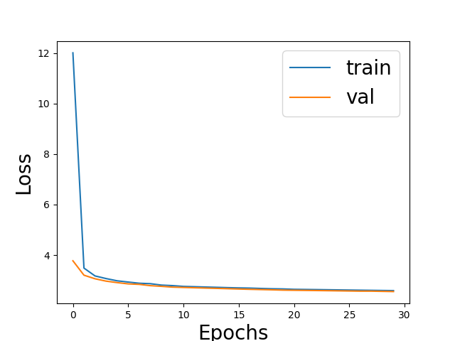
We plot the training loss and validation loss

# Plot
# sphinx_gallery_thumbnail_number = 2

fig = plt.figure()
plt.plot(train_info["train"], label="train")
plt.plot(train_info["val"], label="val")
plt.xlabel("Epochs", fontsize=20)
plt.ylabel("Loss", fontsize=20)
plt.legend(fontsize=20)
plt.show()

Note

See the googlecolab notebook spyrit-examples/tutorial/tuto_train_lin_meas_colab.ipynb for training a reconstruction network on GPU. It shows how to train using different architectures, denoisers and other hyperparameters from train_model() function.