Note
Go to the end to download the full example code.
01. Acquisition operators
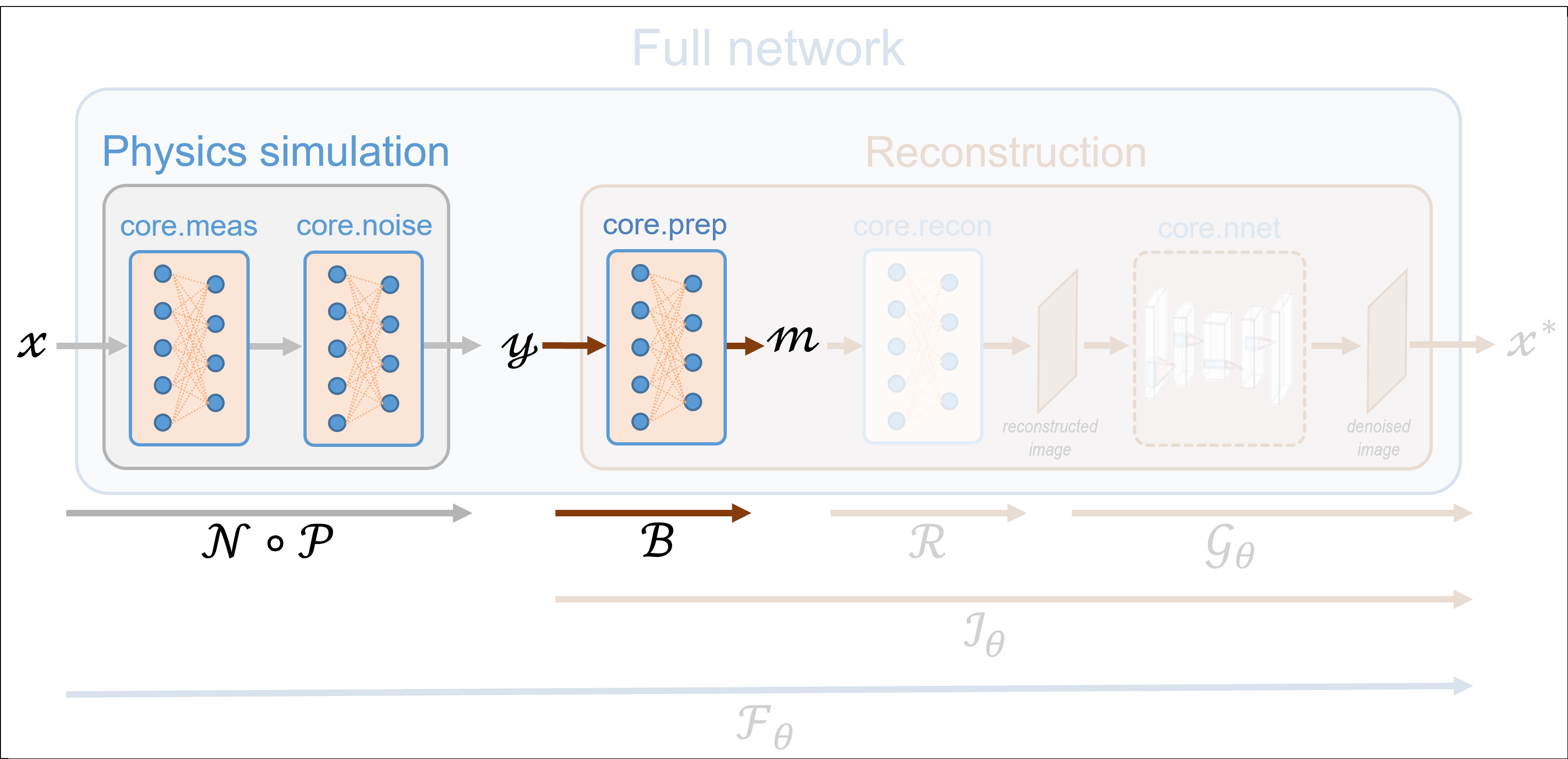
This tutorial shows how to simulate measurements using the spyrit.core
submodule. The simulation is based on three modules:
Measurement operators compute linear measurements \(y = Hx\) from images \(x\), where \(H\) is a linear operator (matrix) and \(x\) is a vectorized image (see
spyrit.core.meas)Noise operator corrupts measurements \(y\) with noise (see
spyrit.core.noise)Preprocessing operators are typically used to process the noisy measurements prior to reconstruction (see
spyrit.core.prep)
These tutorials load image samples from /images/.
Load a batch of images
Images \(x\) for training neural networks expect values in [-1,1]. The images are normalized
using the transform_gray_norm() function.
import os

import torch
import torchvision
import matplotlib.pyplot as plt

from spyrit.misc.disp import imagesc
from spyrit.misc.statistics import transform_gray_norm

# sphinx_gallery_thumbnail_path = 'fig/tuto1.png'

h = 64  # image size hxh
i = 1  # Image index (modify to change the image)
spyritPath = os.getcwd()
imgs_path = os.path.join(spyritPath, "images/")


# Create a transform for natural images to normalized grayscale image tensors
transform = transform_gray_norm(img_size=h)

# Create dataset and loader (expects class folder 'images/test/')
dataset = torchvision.datasets.ImageFolder(root=imgs_path, transform=transform)
dataloader = torch.utils.data.DataLoader(dataset, batch_size=7)

x, _ = next(iter(dataloader))
print(f"Shape of input images: {x.shape}")

# Select image
x = x[i : i + 1, :, :, :]
x = x.detach().clone()
b, c, h, w = x.shape

# plot
x_plot = x.view(-1, h, h).cpu().numpy()
imagesc(x_plot[0, :, :], r"$x$ in [-1, 1]")
![$x$ in [-1, 1]](../_images/sphx_glr_tuto_01_acquisition_operators_001.png)
Shape of input images: torch.Size([7, 1, 64, 64])
The measurement and noise operators
Noise operators are defined in the noise module. A noise
operator computes the following three steps sequentially:
1. Normalization of the image \(x\) with values in [-1,1] to get an image \(\tilde{x}=\frac{x+1}{2}\) in [0,1], as it is required for measurement simulation
Application of the measurement model, i.e., computation of \(H\tilde{x}\)
Application of the noise model
The normalization is usefull when considering distributions such as the Poisson distribution that are defined on positive values.
Note
The noise operator is constructed from a measurement operator (see the
meas submodule) in order to compute the measurements
\(H\tilde{x}\), as given by step #2.
A simple example: identity measurement matrix and no noise
We start with a simple example where the measurement matrix \(H\) is
the identity, which can be handled by the more general
spyrit.core.meas.Linear class. We consider the noiseless case handled
by the spyrit.core.noise.NoNoise class.
We simulate the measurement vector \(y\) that we visualise as an image. Remember that the input image \(x\) is handled as a vector.
![$\tilde{x}$ in [0, 1]](../_images/sphx_glr_tuto_01_acquisition_operators_002.png)
Shape of vectorized image: torch.Size([1, 4096])
Shape of simulated measurements y: torch.Size([1, 4096])
Note
Note that the image identical to the original one, except it has been normalized in [0,1].
Same example with Poisson noise
We now consider Poisson noise, i.e., a noisy measurement vector given by
where \(\alpha\) is a scalar value that represents the maximum image intensity (in photons). The larger \(\alpha\), the higher the signal-to-noise ratio.
We consider the spyrit.core.noise.Poisson class and set \(\alpha\)
to 100 photons.
We simulate two noisy measurement vectors
We now consider the case \(\alpha = 1000\) photons.
We finally plot the measurement vectors as images
# plot
y1_plot = y1.view(b, h, h).detach().numpy()
y2_plot = y2.view(b, h, h).detach().numpy()
y3_plot = y3.view(b, h, h).detach().numpy()

f, axs = plt.subplots(1, 3, figsize=(10, 5))
axs[0].set_title("100 photons")
im = axs[0].imshow(y1_plot[0, :, :], cmap="gray")
add_colorbar(im, "bottom")

axs[1].set_title("100 photons")
im = axs[1].imshow(y2_plot[0, :, :], cmap="gray")
add_colorbar(im, "bottom")

axs[2].set_title("1000 photons")
im = axs[2].imshow(y3_plot[0, :, :], cmap="gray")
add_colorbar(im, "bottom")

noaxis(axs)
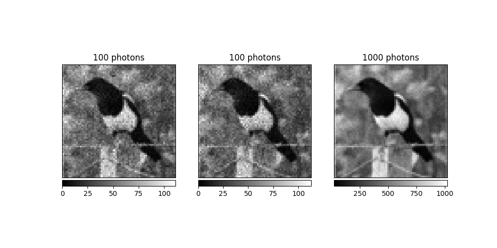
As expected the signal-to-noise ratio of the measurement vector is higher for 1,000 photons than for 100 photons
Note
Not only the signal-to-noise, but also the scale of the measurements depends on \(\alpha\), which motivate the introduction of the preprocessing operator.
The preprocessing operator
Preprocessing operators are defined in the spyrit.core.prep module.
A preprocessing operator applies to the noisy measurements
For instance, a preprocessing operator can be used to compensate for the scaling factors that appear in the measurement or noise operators. In this case, a preprocessing operator is closely linked to its measurement and/or noise operator counterpart. While scaling factors are required to simulate realistic measurements, they are not required for reconstruction.
Preprocessing measurements corrupted by Poisson noise
We consider the spyrit.core.prep.DirectPoisson class that intends
to “undo” the spyrit.core.noise.Poisson class by compensating for:
the scaling that appears when computing Poisson-corrupted measurements
the affine transformation to get images in [0,1] from images in [-1,1]
For this, it computes
We consider the spyrit.core.prep.DirectPoisson class and set \(\alpha\)
to 100 photons.
from spyrit.core.prep import DirectPoisson

alpha = 100  # number of photons
prep_op = DirectPoisson(alpha, meas_op)
We preprocess the first two noisy measurement vectors
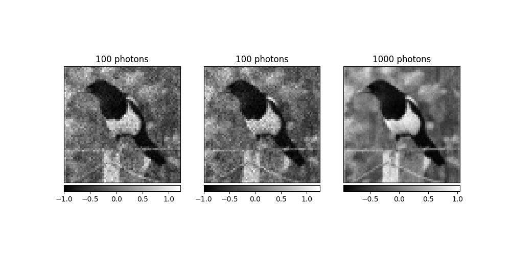
We now consider the case \(\alpha = 1000\) photons to preprocess the third measurement vector
We finally plot the preprocessed measurement vectors as images
# plot
m1 = m1.view(b, h, h).detach().numpy()
m2 = m2.view(b, h, h).detach().numpy()
m3 = m3.view(b, h, h).detach().numpy()

f, axs = plt.subplots(1, 3, figsize=(10, 5))
axs[0].set_title("100 photons")
im = axs[0].imshow(m1[0, :, :], cmap="gray")
add_colorbar(im, "bottom")

axs[1].set_title("100 photons")
im = axs[1].imshow(m2[0, :, :], cmap="gray")
add_colorbar(im, "bottom")

axs[2].set_title("1000 photons")
im = axs[2].imshow(m3[0, :, :], cmap="gray")
add_colorbar(im, "bottom")

noaxis(axs)
Note
The preprocessed measurements still have different the signal-to-noise ratios depending on \(\alpha\); however, they (approximately) all lie within the same range (here, [-1, 1]).
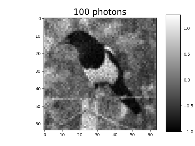
We show again one of the preprocessed measurement vectors (tutorial thumbnail purpose)
# Plot
imagesc(m2[0, :, :], "100 photons", title_fontsize=20)
Total running time of the script: (0 minutes 0.982 seconds)