08. Learned proximal gradient descent (LPGD) for split measurements

This tutorial shows how to perform image reconstruction with unrolled Learned Proximal Gradient Descent (LPGD) for split measurements.

Unfortunately, it has a large memory consumption so it cannot be run interactively. If you want to run it yourself, please remove all the “if False:” statements at the beginning of each code block. The figures displayed are the ones that would be generated if the code was run.

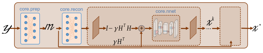
LPGD is a unrolled method, which can be explained as a recurrent network where each block corresponds to un unrolled iteration of the proximal gradient descent. At each iteration, the network performs a gradient step and a denoising step.

The updated rule for the LPGD network is given by:

\[x^{(k+1)} = \mathcal{G}_{\theta}(x^{(k)} - \gamma H^T(H(x^{(k)}-m))).\]

where \(x^{(k)}\) is the image estimate at iteration \(k\), \(H\) is the forward operator, \(\gamma\) is the step size, and \(\mathcal{G}_{\theta}\) is a denoising network with learnable parameters \(\theta\).

Load a batch of images

Images \(x\) for training neural networks expect values in [-1,1]. The images are normalized using the transform_gray_norm() function.

# sphinx_gallery_thumbnail_path = 'fig/lpgd.png'

if False:
    import os

    import torch
    import torchvision
    import numpy as np

    from spyrit.misc.disp import imagesc
    from spyrit.misc.statistics import transform_gray_norm

    h = 128  # image size hxh
    i = 1  # Image index (modify to change the image)
    spyritPath = os.getcwd()
    imgs_path = os.path.join(spyritPath, "images")
    # Create a transform for natural images to normalized grayscale image tensors
    transform = transform_gray_norm(img_size=h)
    # Create dataset and loader (expects class folder 'images/test/')
    dataset = torchvision.datasets.ImageFolder(root=imgs_path, transform=transform)
    dataloader = torch.utils.data.DataLoader(dataset, batch_size=7)

    x, _ = next(iter(dataloader))
    print(f"Shape of input images: {x.shape}")  # torch.Size([7, 1, 128, 128])
    # Select image
    x = x[i : i + 1, :, :, :]
    x = x.detach().clone()
    b, c, h, w = x.shape

    # plot
    x_plot = x.view(-1, h, h).cpu().numpy()
    imagesc(x_plot[0, :, :], r"$x$ in [-1, 1]")

%% Forward operators for split measurements —————————————————————————–

We consider noisy split measurements for a Hadamard operator and a simple rectangular subsampling” strategy (for more details, refer to Acquisition - split measurements).

We define the measurement, noise and preprocessing operators and then simulate a measurement vector \(y\) corrupted by Poisson noise. As in the previous tutorial, we simulate an accelerated acquisition by subsampling the measurement matrix by retaining only the first rows of a Hadamard matrix.

if False:
    import math

    from spyrit.core.meas import HadamSplit
    from spyrit.core.noise import Poisson
    from spyrit.core.prep import SplitPoisson
    from spyrit.misc.sampling import meas2img

    # Measurement parameters
    M = 4096  # Number of measurements (here, 1/4 of the pixels)
    alpha = 10.0  # number of photons

    # Sampling: rectangular matrix
    Ord_rec = np.ones((h, h))
    n_sub = math.ceil(M**0.5)
    Ord_rec[:, n_sub:] = 0
    Ord_rec[n_sub:, :] = 0

    # Measurement and noise operators
    meas_op = HadamSplit(M, h, torch.from_numpy(Ord_rec))
    noise_op = Poisson(meas_op, alpha)
    prep_op = SplitPoisson(alpha, meas_op)

    # Vectorize image
    x = x.view(b * c, h * w)
    print(f"Shape of vectorized image: {x.shape}")  # torch.Size([1, 16384])

    # Measurements
    y = noise_op(x)  # a noisy measurement vector
    m = prep_op(y)  # preprocessed measurement vector

    m_plot = m.detach().numpy()
    m_plot = meas2img(m_plot, Ord_rec)
    imagesc(m_plot[0, :, :], r"Measurements $m$")

We define the LearnedPGD network by providing the measurement, noise and preprocessing operators, the denoiser and other optional parameters to the class spyrit.core.recon.LearnedPGD. The optional parameters include the number of unrolled iterations (iter_stop) and the step size decay factor (step_decay). We choose Unet as the denoiser, as in previous tutorials. For the optional parameters, we use three iterations and a step size decay factor of 0.9, which worked well on this data (this should match the parameters used during training).

if False:
    from spyrit.core.nnet import Unet
    from spyrit.core.recon import LearnedPGD

    # use GPU, if available
    device = torch.device("cuda:0" if torch.cuda.is_available() else "cpu")
    # Define UNet denoiser
    denoi = Unet()
    # Define the LearnedPGD model
    lpgd_net = LearnedPGD(noise_op, prep_op, denoi, iter_stop=3, step_decay=0.9)

Now, we download the pretrained weights and load them into the LPGD network. Unfortunately, the pretrained weights are too heavy (2GB) to be downloaded here. The last figure is nonetheless displayed to show the results.

if False:
    from spyrit.core.train import load_net

    # Download weights
    model_path = "./model"
    if os.path.exists(model_path) is False:
        os.mkdir(model_path)
        print(f"Created {model_path}")

    url_lpgd = "https://drive.google.com/file/d/1ki_cJQEwBWrpDhtE7-HoSEoY8oJUnUz5/view?usp=drive_link"
    model_net_path = os.path.join(
        model_path,
        "lpgd_unet_imagenet_N0_10_m_hadam-split_N_128_M_4096_epo_30_lr_0.001_sss_10_sdr_0.5_bs_128_reg_1e-07_uit_3_sdec0-9.pth",
    )

    if os.path.exists(model_net_path) is False:
        try:
            import gdown

            gdown.download(url_lpgd, model_net_path, quiet=False, fuzzy=True)
        except:
            print(f"Model not downloaded from {url_lpgd}!!!")

    # Load pretrained weights to the model
    load_net(model_net_path, lpgd_net, device, strict=False)

    lpgd_net.eval()
    lpgd_net.to(device)

We reconstruct by calling the reconstruct method as in previous tutorials and display the results.

if False:
    import matplotlib.pyplot as plt

    from spyrit.misc.disp import add_colorbar, noaxis

    with torch.no_grad():
        z_lpgd = lpgd_net.reconstruct(y.to(device))

    # Plot results
    x_plot = x.view(-1, h, h).cpu().numpy()
    x_plot2 = z_lpgd.view(-1, h, h).cpu().numpy()

    f, axs = plt.subplots(2, 1, figsize=(10, 10))
    im1 = axs[0].imshow(x_plot[0, :, :], cmap="gray")
    axs[0].set_title("Ground-truth image", fontsize=16)
    noaxis(axs[0])
    add_colorbar(im1, "bottom")

    im2 = axs[1].imshow(x_plot2[0, :, :], cmap="gray")
    axs[1].set_title("LPGD", fontsize=16)
    noaxis(axs[1])
    add_colorbar(im2, "bottom")

    plt.show()