05. Acquisition operators (advanced) - Split measurements and subsampling

This tutorial is an extension of the Tutorials 01 and 02 where:

• we introduce split measurements to handle a Hadamard measurements,

• we discuss subsampling for accelerated acquisitions.

Load a batch of images

Images \(x\) for training neural networks expect values in [-1,1]. The images are normalized using the transform_gray_norm() function.

import os

import torch
import torchvision
import numpy as np
import matplotlib.pyplot as plt

from spyrit.misc.disp import imagesc
from spyrit.misc.statistics import transform_gray_norm


h = 64  # image size hxh
i = 1  # Image index (modify to change the image)
spyritPath = os.getcwd()
imgs_path = os.path.join(spyritPath, "images/")


# Create a transform for natural images to normalized grayscale image tensors
transform = transform_gray_norm(img_size=h)

# Create dataset and loader (expects class folder 'images/test/')
dataset = torchvision.datasets.ImageFolder(root=imgs_path, transform=transform)
dataloader = torch.utils.data.DataLoader(dataset, batch_size=7)

x, _ = next(iter(dataloader))
print(f"Shape of input images: {x.shape}")

# Select image
x = x[i : i + 1, :, :, :]
x = x.detach().clone()
b, c, h, w = x.shape

# plot
x_plot = x.view(-1, h, h).cpu().numpy()
imagesc(x_plot[0, :, :], r"$x$ in [-1, 1]")

Shape of input images: torch.Size([7, 1, 64, 64])

The measurement and noise operators

Noise operators are defined in the noise module. A noise operator computes the following three steps sequentially:

1. Normalization of the image \(x\) with values in [-1,1] to get an image \(\tilde{x}=\frac{x+1}{2}\) in [0,1], as it is required for measurement simulation

2. Application of the measurement model, i.e., computation of \(P\tilde{x}\)

3. Application of the noise model

\[y \sim \texttt{Noise}(P\tilde{x}) = \texttt{Noise}\left(\frac{P(x+1)}{2}\right).\]

The normalization is useful when considering distributions such as the Poisson distribution that are defined on positive values.

Split measurement operator and no noise

\[\begin{split}y = P\tilde{x}= \begin{bmatrix} H_{+} \\ H_{-} \end{bmatrix} \tilde{x}.\end{split}\]

Hadamard split measurement operator is defined in the spyrit.core.meas.HadamSplit class. It computes linear measurements from incoming images, where \(P\) is a linear operator (matrix) with positive entries and \(\tilde{x}\) is a vectorized image. The class relies on a matrix \(H\) with shape \((M,N)\) where \(N\) represents the number of pixels in the image and \(M \le N\) the number of measurements. The matrix \(P\) is obtained by splitting the matrix \(H\) as \(H = H_{+}-H_{-}\) where \(H_{+} = \max(0,H)\) and \(H_{-} = \max(0,-H)\).

Subsampling

Subsampling is done by retaining the first \(M\) rows of a permuted Hadamard matrix \(H=GF\), where \(G\) is a subsampled permutation matrix with shape \((M,N)\) and \(F\) is a “full” Hadamard matrix with shape \((N,N)\).

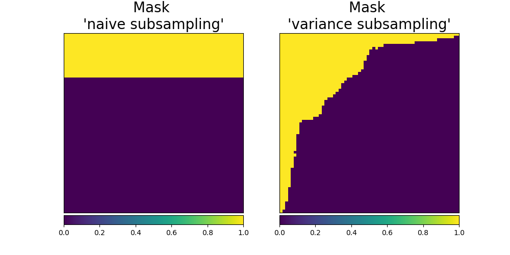
We consider two subsampling strategies:

• “Naive subsampling” by retaining only the first \(M\) rows of the measurement matrix.

• “Variance subsampling” by retaining only the first \(M\) rows of a permuted measurement matrix where the first rows corresponds to the coefficients with largest variance and the last ones to the coefficients that are close to constant. The motivation is that almost constant coefficients are less informative than the others. This can be supported by principal component analysis, which states that preserving the components with largest variance leads to the best linear predictor.

First, we download the covariance matrix from our warehouse and load it. The covariance matrix has been computed from ImageNet 2012 dataset.

import girder_client

# api Rest url of the warehouse
url = "https://pilot-warehouse.creatis.insa-lyon.fr/api/v1"

# Generate the warehouse client
gc = girder_client.GirderClient(apiUrl=url)

# Download the covariance matrix and mean image
data_folder = "./stat/"
dataId_list = [
    "63935b624d15dd536f0484a5",  # for reconstruction (imageNet, 64)
    "63935a224d15dd536f048496",  # for reconstruction (imageNet, 64)
]
cov_name = "./stat/Cov_64x64.npy"

try:
    for dataId in dataId_list:
        myfile = gc.getFile(dataId)
        gc.downloadFile(dataId, data_folder + myfile["name"])

    print(f"Created {data_folder}")

    # Load covariance matrix for "variance subsampling"
    Cov = np.load(cov_name)
    print(f"Cov matrix {cov_name} loaded")
except:
    # Set to the identity if not found for "naive subsampling"
    Cov = np.eye(h * h)
    print(f"Cov matrix {cov_name} not found! Set to the identity")

/home/docs/checkouts/readthedocs.org/user_builds/spyrit/envs/2.3.1/lib/python3.11/site-packages/girder_client/__init__.py:1: DeprecationWarning: pkg_resources is deprecated as an API. See https://setuptools.pypa.io/en/latest/pkg_resources.html
  from pkg_resources import DistributionNotFound, get_distribution
/home/docs/checkouts/readthedocs.org/user_builds/spyrit/envs/2.3.1/lib/python3.11/site-packages/pkg_resources/__init__.py:3117: DeprecationWarning: Deprecated call to `pkg_resources.declare_namespace('sphinxcontrib')`.
Implementing implicit namespace packages (as specified in PEP 420) is preferred to `pkg_resources.declare_namespace`. See https://setuptools.pypa.io/en/latest/references/keywords.html#keyword-namespace-packages
  declare_namespace(pkg)
Created ./stat/
Cov matrix ./stat/Cov_64x64.npy loaded

The permutation matrix is defined from a sampling matrix with shape \((\sqrt{N},\sqrt{N})\) (see the sampling submodule).

We compute the sampling matrix for the “naive” subsampling

from spyrit.misc.statistics import Cov2Var
from spyrit.misc.disp import add_colorbar, noaxis


M = 64 * 64 // 4  # number of measurements (here, 1/4 of the pixels)
Cov_eye = np.eye(h * h)
Ord_nai = Cov2Var(Cov_eye)

And for the “variance” subsampling

Ord_var = Cov2Var(Cov)

Further insight on the two strategies can be gained by plotting the masks corresponding to the sampling matrices.

# sphinx_gallery_thumbnail_number = 2
from spyrit.misc.sampling import sort_by_significance

mask_basis = np.zeros((h, h))
mask_basis.flat[:M] = 1

# Mask for "naive subsampling"
mask_nai = sort_by_significance(mask_basis, Ord_nai, axis="flatten")

# Mask for "variance subsampling"
mask_var = sort_by_significance(mask_basis, Ord_var, axis="flatten")

# Plot the masks
f, (ax1, ax2) = plt.subplots(1, 2, figsize=(10, 5))
im1 = ax1.imshow(mask_nai, vmin=0, vmax=1)
ax1.set_title("Mask \n'naive subsampling'", fontsize=20)
noaxis(ax1)
add_colorbar(im1, "bottom", size="20%")

im2 = ax2.imshow(mask_var, vmin=0, vmax=1)
ax2.set_title("Mask \n'variance subsampling'", fontsize=20)
noaxis(ax2)
add_colorbar(im2, "bottom", size="20%")

<matplotlib.colorbar.Colorbar object at 0x7f8c6affea10>

Note

Note that in this tutorial the covariance matrix is used only for choosing the subsampling strategy. Although the covariance matrix can be also exploited to improve the reconstruction, this will be considered in a future tutorial.

Measurement and noise operators

We compute the measurement and noise operators and then simulate the measurement vector \(y\).

We consider Poisson noise, i.e., a noisy measurement vector given by

\[y \sim \mathcal{P}(\alpha P \tilde{x}),\]

where \(\alpha\) is a scalar value that represents the maximum image intensity (in photons). The larger \(\alpha\), the higher the signal-to-noise ratio.

We use the spyrit.core.noise.Poisson class, set \(\alpha\) to 100 photons, and simulate a noisy measurement vector for the two sampling strategies. Subsampling is handled internally by the HadamSplit class.

from spyrit.core.noise import Poisson
from spyrit.core.meas import HadamSplit
from spyrit.core.noise import Poisson

alpha = 100.0  # number of photons

# "Naive subsampling"
# Measurement and noise operators
meas_nai_op = HadamSplit(M, h, torch.from_numpy(Ord_nai))
noise_nai_op = Poisson(meas_nai_op, alpha)

# Measurement operator
x = x.view(b * c, h * w)  # vectorized image
y_nai = noise_nai_op(x)  # a noisy measurement vector

# "Variance subsampling"
meas_var_op = HadamSplit(M, h, torch.from_numpy(Ord_var))
noise_var_op = Poisson(meas_var_op, alpha)
y_var = noise_var_op(x)  # a noisy measurement vector

x = x.view(b * c, h * w)  # vectorized image
print(f"Shape of vectorized image: {x.shape}")
print(f"Shape of simulated measurements y: {y_var.shape}")

Shape of vectorized image: torch.Size([1, 4096])
Shape of simulated measurements y: torch.Size([1, 2048])

The preprocessing operator measurements for split measurements

We compute the preprocessing operators for the three cases considered above, using the spyrit.core.prep module. As previously introduced, a preprocessing operator applies to the noisy measurements in order to compensate for the scaling factors that appear in the measurement or noise operators:

\[m = \texttt{Prep}(y),\]

We consider the spyrit.core.prep.SplitPoisson class that intends to “undo” the spyrit.core.noise.Poisson class, for split measurements, by compensating for

• the scaling that appears when computing Poisson-corrupted measurements

• the affine transformation to get images in [0,1] from images in [-1,1]

For this, it computes

\[m = \frac{2(y_+-y_-)}{\alpha} - P\mathbb{1},\]

where \(y_+=H_+\tilde{x}\) and \(y_-=H_-\tilde{x}\). This is handled internally by the spyrit.core.prep.SplitPoisson class.

We compute the preprocessing operator and the measurements vectors for the two sampling strategies.

from spyrit.core.prep import SplitPoisson

# "Naive subsampling"
#
# Preprocessing operator
prep_nai_op = SplitPoisson(alpha, meas_nai_op)

# Preprocessed measurements
m_nai = prep_nai_op(y_nai)

# "Variance subsampling"
prep_var_op = SplitPoisson(alpha, meas_var_op)
m_var = prep_var_op(y_var)

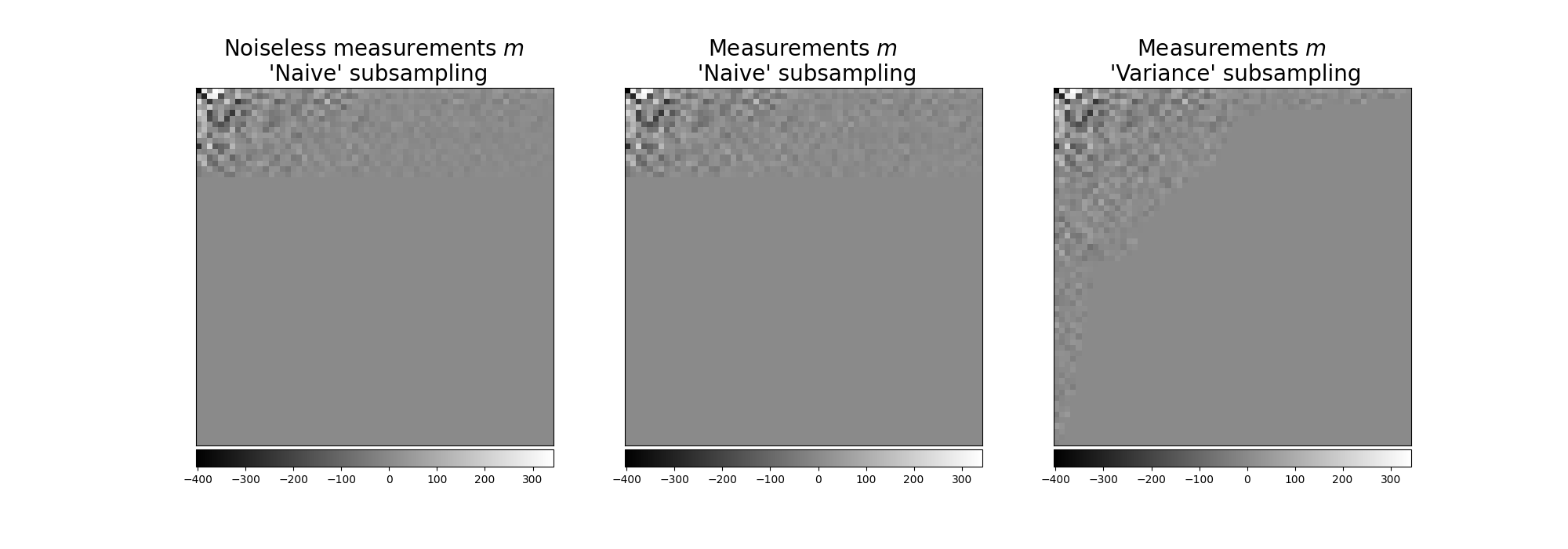
Noiseless measurements

We consider now noiseless measurements for the “naive subsampling” strategy. We compute the required operators and the noiseless measurement vector. For this we use the spyrit.core.noise.NoNoise class, which normalizes the input vector to get an image in [0,1], as explained in acquisition operators tutorial. For the preprocessing operator, we assign the number of photons equal to one.

from spyrit.core.noise import NoNoise

nonoise_nai_op = NoNoise(meas_nai_op)
y_nai_nonoise = nonoise_nai_op(x)  # a noisy measurement vector

prep_nonoise_op = SplitPoisson(1.0, meas_nai_op)
m_nai_nonoise = prep_nonoise_op(y_nai_nonoise)

We can now plot the three measurement vectors

from spyrit.misc.sampling import meas2img

# Plot the three measurement vectors
m_plot = m_nai_nonoise.numpy()
m_plot = meas2img(m_plot, Ord_nai)
m_plot_max = np.max(m_plot[0, :, :])
m_plot_min = np.min(m_plot[0, :, :])

m_plot2 = m_nai.numpy()
m_plot2 = meas2img(m_plot2, Ord_nai)

m_plot3 = m_var.numpy()
m_plot3 = meas2img(m_plot3, Ord_var)

f, (ax1, ax2, ax3) = plt.subplots(1, 3, figsize=(20, 7))
im1 = ax1.imshow(m_plot[0, :, :], cmap="gray")
ax1.set_title("Noiseless measurements $m$ \n 'Naive' subsampling", fontsize=20)
noaxis(ax1)
add_colorbar(im1, "bottom", size="20%")

im2 = ax2.imshow(m_plot2[0, :, :], cmap="gray", vmin=m_plot_min, vmax=m_plot_max)
ax2.set_title("Measurements $m$ \n 'Naive' subsampling", fontsize=20)
noaxis(ax2)
add_colorbar(im2, "bottom", size="20%")

im3 = ax3.imshow(m_plot3[0, :, :], cmap="gray", vmin=m_plot_min, vmax=m_plot_max)
ax3.set_title("Measurements $m$ \n 'Variance' subsampling", fontsize=20)
noaxis(ax3)
add_colorbar(im3, "bottom", size="20%")

<matplotlib.colorbar.Colorbar object at 0x7f8c68d89910>

PinvNet network

We use the spyrit.core.recon.PinvNet class where the pseudo inverse reconstruction is performed by a neural network

from spyrit.core.recon import PinvNet

# PinvNet(meas_op, prep_op, denoi=torch.nn.Identity())
pinvnet_nai_nonoise = PinvNet(nonoise_nai_op, prep_nonoise_op)
pinvnet_nai = PinvNet(noise_nai_op, prep_nai_op)
pinvnet_var = PinvNet(noise_var_op, prep_var_op)

# Reconstruction
z_nai_nonoise = pinvnet_nai_nonoise.reconstruct(y_nai_nonoise)
z_nai = pinvnet_nai.reconstruct(y_nai)
z_var = pinvnet_var.reconstruct(y_var)

We can now plot the three reconstructed images

from spyrit.misc.disp import add_colorbar, noaxis

# Plot
x_plot = x.view(-1, h, h).numpy()
z_plot_nai_nonoise = z_nai_nonoise.view(-1, h, h).numpy()
z_plot_nai = z_nai.view(-1, h, h).numpy()
z_plot_var = z_var.view(-1, h, h).numpy()

f, axs = plt.subplots(2, 2, figsize=(10, 10))
im1 = axs[0, 0].imshow(x_plot[0, :, :], cmap="gray")
axs[0, 0].set_title("Ground-truth image")
noaxis(axs[0, 0])
add_colorbar(im1, "bottom")

im2 = axs[0, 1].imshow(z_plot_nai_nonoise[0, :, :], cmap="gray")
axs[0, 1].set_title("Reconstruction noiseless")
noaxis(axs[0, 1])
add_colorbar(im2, "bottom")

im3 = axs[1, 0].imshow(z_plot_nai[0, :, :], cmap="gray")
axs[1, 0].set_title("Reconstruction \n 'Naive' subsampling")
noaxis(axs[1, 0])
add_colorbar(im3, "bottom")

im4 = axs[1, 1].imshow(z_plot_var[0, :, :], cmap="gray")
axs[1, 1].set_title("Reconstruction \n 'Variance' subsampling")
noaxis(axs[1, 1])
add_colorbar(im4, "bottom")

plt.show()

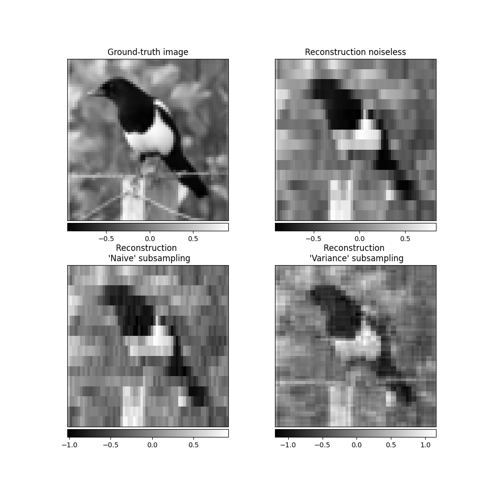
Note

Note that reconstructed images are pixelized when using the “naive subsampling”, while they are smoother and more similar to the ground-truth image when using the “variance subsampling”.

Another way to further improve results is to include a nonlinear post-processing step, which we will consider in a future tutorial.