02. Pseudoinverse solution from linear measurements

This tutorial shows how to simulate measurements and perform image reconstruction. The measurement operator is chosen as a Hadamard matrix with positive coefficients. Note that this matrix can be replaced by any desired matrix.

These tutorials load image samples from /images/.

Load a batch of images

Images \(x\) for training expect values in [-1,1]. The images are normalized using the transform_gray_norm() function.

import os

import torch
import torchvision
import numpy as np

from spyrit.misc.disp import imagesc
from spyrit.misc.statistics import transform_gray_norm

# sphinx_gallery_thumbnail_path = 'fig/tuto2.png'

h = 64  # image size hxh
i = 1  # Image index (modify to change the image)
spyritPath = os.getcwd()
imgs_path = os.path.join(spyritPath, "images/")


# Create a transform for natural images to normalized grayscale image tensors
transform = transform_gray_norm(img_size=h)

# Create dataset and loader (expects class folder 'images/test/')
dataset = torchvision.datasets.ImageFolder(root=imgs_path, transform=transform)
dataloader = torch.utils.data.DataLoader(dataset, batch_size=7)

x, _ = next(iter(dataloader))
print(f"Shape of input images: {x.shape}")

# Select image
x = x[i : i + 1, :, :, :]
x = x.detach().clone()
b, c, h, w = x.shape

# plot
x_plot = x.view(-1, h, h).cpu().numpy()
imagesc(x_plot[0, :, :], r"$x$ in [-1, 1]")

Shape of input images: torch.Size([7, 1, 64, 64])

Define a measurement operator

We consider the case where the measurement matrix is the positive component of a Hadamard matrix, which is often used in single-pixel imaging. First, we compute a full Hadamard matrix that computes the 2D transform of an image of size h and takes its positive part.

from spyrit.misc.walsh_hadamard import walsh2_matrix

F = walsh2_matrix(h)
F = np.where(F > 0, F, 0)

Next, we subsample the rows of the measurement matrix to simulate an accelerated acquisition. For this, we use the spyrit.misc.sampling.sort_by_significance() function that returns an input matrix whose rows are ordered in increasing order of significance according to a given array. The array is a sampling map that indicates the location of the most significant coefficients in the transformed domain.

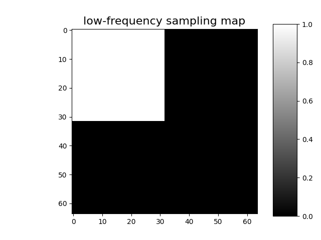
To keep the low-frequency Hadamard coefficients, we choose a sampling map with ones in the top left corner and zeros elsewhere.

import math

und = 4  # undersampling factor
M = h**2 // und  # number of measurements (undersampling factor = 4)

Sampling_map = np.ones((h, h))
M_xy = math.ceil(M**0.5)
Sampling_map[:, M_xy:] = 0
Sampling_map[M_xy:, :] = 0

imagesc(Sampling_map, "low-frequency sampling map")

After permutation of the full Hadamard matrix, we keep only its first M rows

from spyrit.misc.sampling import sort_by_significance

F = sort_by_significance(F, Sampling_map, "rows", False)
H = F[:M, :]

print(f"Shape of the measurement matrix: {H.shape}")

Shape of the measurement matrix: (1024, 4096)

Then, we instantiate a spyrit.core.meas.Linear measurement operator

from spyrit.core.meas import Linear

meas_op = Linear(torch.from_numpy(H), pinv=True)

Noiseless case

In the noiseless case, we consider the spyrit.core.noise.NoNoise noise operator

from spyrit.core.noise import NoNoise

noise = NoNoise(meas_op)

# Simulate measurements
y = noise(x.view(b * c, h * w))
print(f"Shape of raw measurements: {y.shape}")

Shape of raw measurements: torch.Size([1, 1024])

To display the subsampled measurement vector as an image in the transformed domain, we use the spyrit.misc.sampling.meas2img() function

# plot
from spyrit.misc.sampling import meas2img

y_plot = y.detach().numpy().squeeze()
y_plot = meas2img(y_plot, Sampling_map)
print(f"Shape of the raw measurement image: {y_plot.shape}")

imagesc(y_plot, "Raw measurements (no noise)")

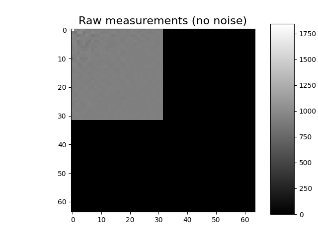
Shape of the raw measurement image: (64, 64)

We now compute and plot the preprocessed measurements corresponding to an image in [-1,1]. For details in the preprocessing, see Tutorial 1.

Note

Using spyrit.core.prep.DirectPoisson with \(\alpha = 1\) allows to compensate for the image normalisation achieved by spyrit.core.noise.NoNoise.

from spyrit.core.prep import DirectPoisson

prep = DirectPoisson(1.0, meas_op)  # "Undo" the NoNoise operator

m = prep(y)
print(f"Shape of the preprocessed measurements: {m.shape}")

# plot
m_plot = m.detach().numpy().squeeze()
m_plot = meas2img(m_plot, Sampling_map)
print(f"Shape of the preprocessed measurement image: {m_plot.shape}")

imagesc(m_plot, "Preprocessed measurements (no noise)")

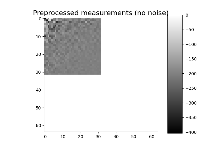
Shape of the preprocessed measurements: torch.Size([1, 1024])
Shape of the preprocessed measurement image: (64, 64)

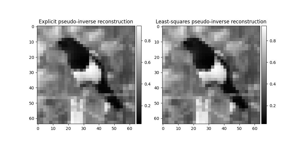
Pseudo inverse

There are two ways to perform the pseudo inverse reconstruction from the measurements y. The first consists of explicitly computing the pseudo inverse of the measurement matrix H and applying it to the measurements. The second computes a least-squares solution using torch.linalg.lstsq() to compute the pseudo inverse solution. The choice is made automatically: if the measurement operator has a pseudo-inverse already computed, it is used; otherwise, the least-squares solution is used.

Note

Generally, the second method is preferred because it is faster and more numerically stable. However, if you will use the pseudo inverse multiple times, it becomes more efficient to compute it explicitly.

First way: explicit computation of the pseudo inverse We can use the spyrit.core.recon.PseudoInverse class to perform the pseudo inverse reconstruction from the measurements y.

from spyrit.core.recon import PseudoInverse

# Pseudo-inverse reconstruction operator
recon_op = PseudoInverse()

# Reconstruction
x_rec1 = recon_op(y, meas_op)  # equivalent to: meas_op.pinv(y)

Second way: calling pinv method from the Linear operator The code is very similar to the previous case, but we need to make sure the measurement operator has no pseudo-inverse computed. We can also specify regularization parameters for the least-squares solution when calling recon_op.

print(f"Pseudo-inverse computed: {hasattr(meas_op, 'H_pinv')}")
temp = meas_op.H_pinv  # save the pseudo-inverse
del meas_op.H_pinv  # delete the pseudo-inverse
print(f"Pseudo-inverse computed: {hasattr(meas_op, 'H_pinv')}")

# Reconstruction
x_rec2 = recon_op(y, meas_op, reg="L1", eta=1e-6)

# restore the pseudo-inverse
meas_op.H_pinv = temp

Pseudo-inverse computed: True
Pseudo-inverse computed: False

Note

This choice is also offered for dynamic measurement operators which are explained in Tutorial 9.

# plot side by side
import matplotlib.pyplot as plt
from spyrit.misc.disp import add_colorbar

x_plot1 = x_rec1.squeeze().view(h, h).cpu().numpy()
x_plot2 = x_rec2.squeeze().view(h, h).cpu().numpy()

fig, (ax1, ax2) = plt.subplots(1, 2, figsize=(10, 5))

im1 = ax1.imshow(x_plot1, cmap="gray")
ax1.set_title("Explicit pseudo-inverse reconstruction")
add_colorbar(im1, "right", size="20%")

im2 = ax2.imshow(x_plot2, cmap="gray")
ax2.set_title("Least-squares pseudo-inverse reconstruction")
add_colorbar(im2, "right", size="20%")

<matplotlib.colorbar.Colorbar object at 0x7f8c6d206650>

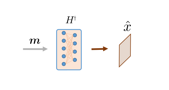
PinvNet Network

Alternatively, we can consider the spyrit.core.recon.PinvNet class that reconstructs an image by computing the pseudoinverse solution, which is fed to a neural networker denoiser. To compute the pseudoinverse solution only, the denoiser can be set to the identity operator

from spyrit.core.recon import PinvNet

pinv_net = PinvNet(noise, prep, denoi=torch.nn.Identity())

or equivalently

pinv_net = PinvNet(noise, prep)

Then, we reconstruct the image from the measurement vector y using the reconstruct() method

x_rec = pinv_net.reconstruct(y)

# plot
x_plot = x_rec.squeeze().cpu().numpy()
imagesc(x_plot, "PinvNet reconstruction (no noise)", title_fontsize=20)

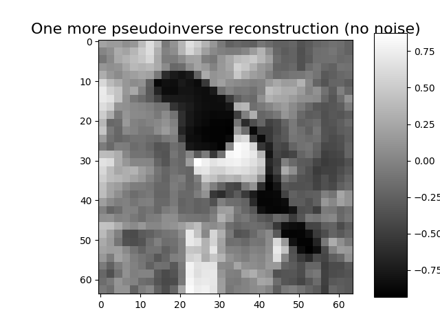
Alternatively, the measurement vector can be simulated using the acquire() method

y = pinv_net.acquire(x)
x_rec = pinv_net.reconstruct(y)

# plot
x_plot = x_rec.squeeze().cpu().numpy()
imagesc(x_plot, "Another pseudoinverse reconstruction (no noise)")

Note that the full module pinv_net both simulates noisy measurements and reconstruct them

x_rec = pinv_net(x)
print(f"Ground-truth image x: {x.shape}")
print(f"Reconstructed x_rec: {x_rec.shape}")

# plot
x_plot = x_rec.squeeze().cpu().numpy()
imagesc(x_plot, "One more pseudoinverse reconstruction (no noise)")

Ground-truth image x: torch.Size([1, 1, 64, 64])
Reconstructed x_rec: torch.Size([1, 1, 64, 64])

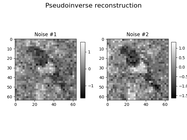
Poisson-corrupted measurement

Here, we consider the spyrit.core.noise.Poisson class together with a spyrit.core.prep.DirectPoisson preprocessing operator (see Tutorial 1).

alpha = 10  # maximum number of photons in the image

from spyrit.core.noise import Poisson
from spyrit.misc.disp import imagecomp

noise = Poisson(meas_op, alpha)
prep = DirectPoisson(alpha, meas_op)  # To undo the "Poisson" operator
pinv_net = PinvNet(noise, prep)

x_rec_1 = pinv_net(x)
x_rec_2 = pinv_net(x)
print(f"Ground-truth image x: {x.shape}")
print(f"Reconstructed x_rec: {x_rec.shape}")

# plot
x_plot_1 = x_rec_1.squeeze().cpu().numpy()
x_plot_1[:2, :2] = 0.0  # hide the top left "crazy pixel" that collects noise
x_plot_2 = x_rec_2.squeeze().cpu().numpy()
x_plot_2[:2, :2] = 0.0  # hide the top left "crazy pixel" that collects noise
imagecomp(x_plot_1, x_plot_2, "Pseudoinverse reconstruction", "Noise #1", "Noise #2")

Ground-truth image x: torch.Size([1, 1, 64, 64])
Reconstructed x_rec: torch.Size([1, 1, 64, 64])

As shown in the next tutorial, a denoising neural network can be trained to postprocess the pseudo inverse solution.