04.b. Pseudoinverse + CNN (training)

This tutorial trains a post processing CNN used by a spyrit.core.recon.PinvNet (see the previous tutorial).

For post-processing, we consider a small CNN; however, it be replaced by any other network (e.g., a Unet). Training is performed on the STL-10 dataset, but any other database can be considered.

You can use Tensorboard for Pytorch for experiment tracking and for visualizing the training process: losses, network weights, and intermediate results (reconstructed images at different epochs).

Measurement operator

We choose the acquisition matrix as the positive component of a Hadamard matrix in “2D”. We subsample it by a factor four, keeping only the low-frequency components (see Tutorial 4 for details).

Positive component of a Hadamard matrix in “2D”.

import torch
from spyrit.core.torch import walsh_matrix_2d

H = walsh_matrix_2d(64)
H = torch.where(H > 0, 1.0, 0.0)

Subsampling map

Sampling_square = torch.zeros(64, 64)
Sampling_square[:32, :32] = 1

Permutation of the rows and subsampling

from spyrit.core.torch import sort_by_significance

H = sort_by_significance(H, Sampling_square, "rows", False)
H = H[: 32 * 32, :]

Associated spyrit.core.meas.Linear operator

from spyrit.core.meas import Linear

# Send to GPU if available
device = torch.device("cuda:0" if torch.cuda.is_available() else "cpu")

meas_op = Linear(H, (64, 64), device=device)

Note

The linear measurement operator is chosen as the positive part of a subsampled Hadamard matrix, but any other matrix can be used.

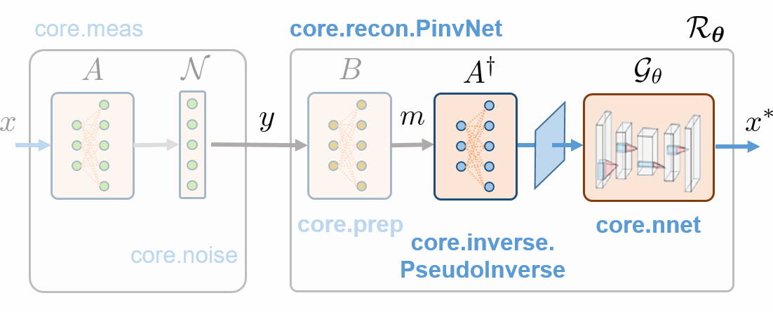
Pseudo inverse solution followed by a CNN

We consider the spyrit.core.recon.PinvNet class that reconstructs an image by computing the pseudoinverse solution and applies a nonlinear network denoiser. First, we must define the denoiser. As an example, we choose a small CNN using the spyrit.core.nnet.ConvNet class. Then, we define the PinvNet network by passing the noise and preprocessing operators and the denoiser.

from typing import OrderedDict
from spyrit.core.nnet import ConvNet

denoiser = torch.nn.Sequential(OrderedDict({"denoi": ConvNet()}))

Note

Here, we consider a small CNN; however, it be replaced by any other network (e.g., a Unet).

We instantiate a spyrit.core.recon.PinvNet with the CNN as an image-domain post processing

from spyrit.core.recon import PinvNet

pinv_net = PinvNet(meas_op, denoi=denoiser, device=device, store_H_pinv=True)

Important

We use store_H_pinv=True to compute and store the pseudo inverse matrix. This will be much faster that using a solver (default option) when a large number of pseudoinverse solutions will have to be computed during training.

Dataloader for training

We now consider the STL10 dataset and use the the normalize=False argument to keep images with values in (0,1).

Set mode_run=True in the the script below to download the STL10 dataset and train the CNN. Otherwise, the CNN paramameters will be downloaded.

# import torch.nn
from spyrit.misc.statistics import data_loaders_stl10
from pathlib import Path

# Parameters
h = 64  # image size hxh
data_root = Path("./data/")  # path to data folder (where the dataset is stored)
batch_size = 700

# Dataloader for STL-10 dataset
mode_run = False
if mode_run:
    dataloaders = data_loaders_stl10(
        data_root,
        img_size=h,
        batch_size=batch_size,
        seed=7,
        shuffle=True,
        download=True,
        normalize=False,
    )

Note

Here, training is performed on the STL-10 dataset, but any other database can be considered.

Optimizer

We define a loss function (mean squared error), an optimizer (Adam) and a scheduler. The scheduler decreases the learning rate by a factor of gamma every step_size epochs.

from spyrit.core.train import Weight_Decay_Loss

# Parameters
lr = 1e-3
step_size = 10
gamma = 0.5

loss = torch.nn.MSELoss()
criterion = Weight_Decay_Loss(loss)
optimizer = torch.optim.Adam(pinv_net.parameters(), lr=lr)
scheduler = torch.optim.lr_scheduler.StepLR(optimizer, step_size=step_size, gamma=gamma)

Training

We use the spyrit.core.train.train_model() function, which iterates through the dataloader, feeds the STL10 images to the full network and optimizes the parameters of the CNN. In addition, it computes the loss and desired metrics on the training and validation sets at each iteration. The training process can be monitored using Tensorboard.

Set mode_run=True to train the CNN (e.g., around 60 min for 20 epochs on my laptop equipped with a NVIDIA Quadro P1000). Otherwise, download the CNN parameters.

from spyrit.core.train import train_model
from datetime import datetime

# Parameters
model_root = Path("./model")  # path to model saving files
num_epochs = 20  # number of training epochs (num_epochs = 30)
checkpoint_interval = 0  # interval between saving model checkpoints
tb_freq = (
    50  # interval between logging to Tensorboard (iterations through the dataloader)
)

# Path for Tensorboard experiment tracking logs
name_run = "stl10_hadam_positive"
now = datetime.now().strftime("%Y-%m-%d_%H-%M")
tb_path = f"runs/runs_{name_run}_nonoise_m{meas_op.M}/{now}"

# Train the network
if mode_run:
    pinv_net, train_info = train_model(
        pinv_net,
        criterion,
        optimizer,
        scheduler,
        dataloaders,
        device,
        model_root,
        num_epochs=num_epochs,
        disp=True,
        do_checkpoint=checkpoint_interval,
        tb_path=tb_path,
        tb_freq=tb_freq,
    )
else:
    train_info = {}

Note

To launch Tensorboard type in a new console:

tensorboard –logdir runs

and open the provided link in a browser. The training process can be monitored in real time in the “Scalars” tab. The “Images” tab allows to visualize the reconstructed images at different iterations tb_freq.

Training history

We save the model so that it can later be utilized. We save the network’s architecture, the training parameters and the training history.

from spyrit.core.train import save_net

title = "tuto_4b"

Path(model_root).mkdir(parents=True, exist_ok=True)
model_path = model_root / (title + ".pth")
train_path = model_root / (title + ".pkl")

if checkpoint_interval:
    Path(model_path).mkdir(parents=True, exist_ok=True)

save_net(model_path, pinv_net.denoi)
# save_net(model_root/(title+"_cnn.pth"), pinv_net.denoi.denoi)

# Save training history
import pickle

if mode_run:
    from spyrit.core.train import Train_par

    reg = 1e-7  # Default value
    params = Train_par(batch_size, lr, h, reg=reg)
    params.set_loss(train_info)

    train_path = model_root / (title + ".pkl")

    with open(train_path, "wb") as param_file:
        pickle.dump(params, param_file)
    torch.cuda.empty_cache()

else:
    from spyrit.misc.load_data import download_girder

    url = "https://tomoradio-warehouse.creatis.insa-lyon.fr/api/v1"
    dataID = "68639a2af39e1d2884b09abc"  # unique ID of the file

    download_girder(url, dataID, model_root)

    with open(train_path, "rb") as param_file:
        params = pickle.load(param_file)

    train_info["train"] = params.train_loss
    train_info["val"] = params.val_loss

model/tuto_4b.pth
Model Saved
Downloading tuto_4b.pkl...
Downloading tuto_4b.pkl... done.

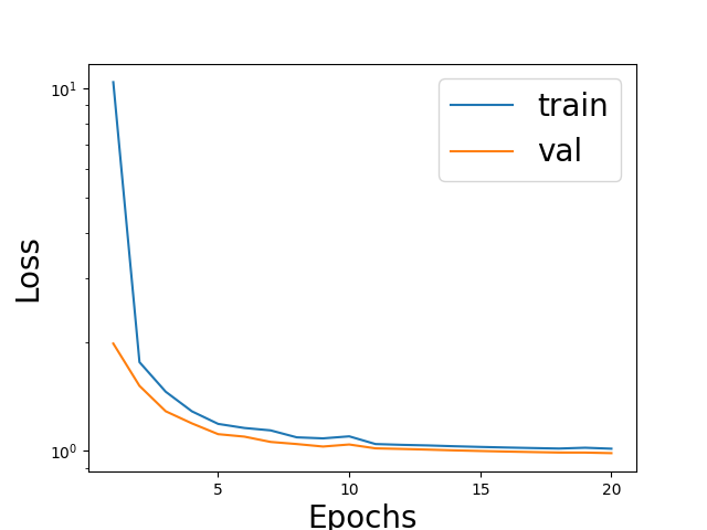
Validation and training losses

We plot the training loss and validation loss

import matplotlib.pyplot as plt
import numpy as np

epoch = np.arange(1, num_epochs + 1)

fig = plt.figure()
plt.semilogy(epoch, train_info["train"], label="train")
plt.semilogy(epoch, train_info["val"], label="val")
plt.xticks([5, 10, 15, 20])
plt.xlabel("Epochs", fontsize=20)
plt.ylabel("Loss", fontsize=20)
plt.legend(fontsize=20)
plt.show()