Note
Go to the end to download the full example code.
06.a. Deformation fields
This tutorial demonstrates how to create and apply deformation fields to
simulate motion in images using the SpyRIT library.
It based on the spyrit.core.warp submodule.
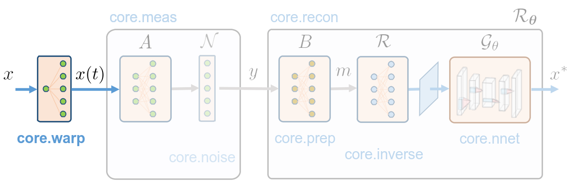
Given a reference image \(x\) and a deformation field \(u(t, :, :)\), it computes the motion video x(t, :, :) by applying the deformation field to the reference image:
Topics covered:
Creating affine deformation fields (translation, rotation, scaling)
Creating elastic deformation fields for realistic motion
Visualizing deformed image sequences
import torch
import torchvision
import matplotlib.pyplot as plt
import math

from pathlib import Path

from spyrit.misc.statistics import transform_norm
from spyrit.misc.load_data import download_girder

from spyrit.core.warp import AffineDeformationField, ElasticDeformation
Set parameters:
thumbnail = True  # True for displaying the motion as a thumbnail, False for a video visualization

n = 64  # size of the FOV side in pixels
img_size = 88  # full image side's size in pixels
n_frames = 50  # number of frames in the dynamic sequence

device = torch.device("cuda" if torch.cuda.is_available() else "cpu")
print("Using device:", device)

dtype = torch.float64
simu_interp = "bilinear"  # interpolation order for motion simulation

time_dim = 1  # time dimension index in tensors

fov_shape = (n, n)
img_shape = (img_size, img_size)
amp_max = (img_shape[0] - fov_shape[0]) // 2
Using device: cpu
Load an image from Tomoradio’s warehouse.
# Download an RGB brain surface image.
url_tomoradio = "https://tomoradio-warehouse.creatis.insa-lyon.fr/api/v1"
data_root = Path("../data/data_online/2025_dynamic")  # local path to data
imgs_path = data_root / Path("images/")
id_files = ["69248e3204d23f6e964b16b7"]  # brain_surface_colorized.png
try:
    download_girder(url_tomoradio, id_files, imgs_path)
except Exception as e:
    print("Unable to download from the Tomoradio warehouse")
    print(e)

# Create a transform for natural images to normalized image tensors
transform = transform_norm(img_size=img_size)
batch_size = 1

# Create dataset and loader
dataset = torchvision.datasets.ImageFolder(root=data_root, transform=transform)
dataloader = torch.utils.data.DataLoader(dataset, batch_size=batch_size)

img, _ = dataloader.dataset[0]
x = img.unsqueeze(0).to(dtype=dtype, device=device)

print(f"Shape of input images: {x.shape}")

x = (x - x.min()) / (x.max() - x.min())  # normalize to [0, 1]
n_wav = x.shape[1]
Local folder not found, creating it... done.
Downloading brain_surface_colorized.png...
Downloading brain_surface_colorized.png... done.
Shape of input images: torch.Size([1, 3, 88, 88])
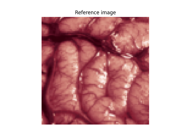
Plot the reference image
x_plot = x.moveaxis(1, -1).squeeze().cpu().numpy()

plt.imshow(x_plot)
if n_wav == 1:
    plt.colorbar(fraction=0.046, pad=0.04)
plt.title("Reference image")
plt.axis("off")
plt.show()
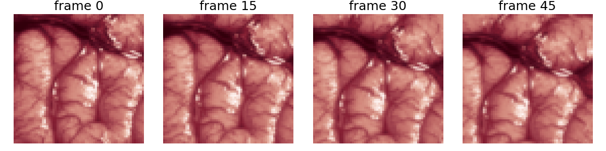
Affine deformation
- Affine deformation examples:
Translation (diagonal motion)
Rotation (spinning motion)
Surface-preserving scaling (pulsating motion)
Important
SpyRIT uses normalized coordinates [-1, 1].
To convert pixels to normalized: normalized = 2 * pixels / image_size
1. Translation (diagonal motion)
T = 1000  # time of a period
time_vector = torch.linspace(0, 2 * T, n_frames)


def translation(t):
    """Translation transformation - diagonal movement."""
    d_pix_tot = 10  # amplitude of translation in pixels
    assert d_pix_tot < amp_max, "Translation amplitude too large for image size!"
    d_normalized = 2 * d_pix_tot / img_size  # Convert to normalized coordinates

    d_pix_unit = d_normalized / (
        2 * T
    )  # normalized amplitude per time unit (for a time vector of length 2T)
    tx = d_pix_unit * t
    ty = -d_pix_unit * t

    return torch.tensor(
        [
            [1, 0, tx],
            [0, 1, ty],
            [0, 0, 1],
        ],
        dtype=dtype,
    )


def_field = AffineDeformationField(
    translation, time_vector, img_shape, dtype=dtype, device=device
)
Simulate motion
x_motion = def_field(x, 0, n_frames, mode=simu_interp)

x_motion = x_motion.moveaxis(time_dim, 1)
print("x_motion.shape:", x_motion.shape)
x_motion.shape: torch.Size([1, 50, 3, 88, 88])
Display deformation within the FOV
if thumbnail:
    # plot few frames as thumbnails
    n_frames_display = 15
    n_rows, n_cols = 1, 4
    plt.figure(figsize=(12, 3))
    for frame in range(n_frames):
        n_frame = n_frames_display * frame
        if n_frame >= n_frames or frame >= n_rows * n_cols:
            break
        plt.subplot(n_rows, n_cols, frame + 1)
        plt.imshow(
            x_motion[
                0,
                n_frame,
                :,
                amp_max : img_size - amp_max,
                amp_max : img_size - amp_max,
            ]
            .moveaxis(0, -1)
            .view(*fov_shape, n_wav)
            .cpu()
            .numpy(),
            cmap="gray",
        )  # in X
        plt.title("frame %d" % (n_frame), fontsize=18)
        plt.axis("off")
    plt.tight_layout()
    plt.show()
else:
    # show motion as video with IPython display
    from IPython.display import clear_output

    n_frames_display = 5
    x_min, x_max = x_motion.min().item(), x_motion.max().item()
    for frame in range(n_frames):
        n_frame = n_frames_display * frame
        if n_frame >= n_frames:
            break
        plt.close()
        plt.imshow(
            x_motion[
                0,
                n_frame,
                :,
                amp_max : img_size - amp_max,
                amp_max : img_size - amp_max,
            ]
            .moveaxis(0, -1)
            .view(*fov_shape, n_wav)
            .cpu()
            .numpy(),
            cmap="gray",
            vmin=x_min,
            vmax=x_max,
        )  # in X
        plt.suptitle("frame %d" % (n_frame), fontsize=16)
        plt.pause(0.1)
        clear_output(wait=True)
2. Rotation (spinning motion)
T = 1000  # time of a period
time_vector = torch.linspace(0, 2 * T, n_frames)


def rotation(t):
    """Rotation transformation - spinning motion."""
    theta = 2 * math.pi * t / T  # One full rotation per period T
    return torch.tensor(
        [
            [math.cos(theta), -math.sin(theta), 0],
            [math.sin(theta), math.cos(theta), 0],
            [0, 0, 1],
        ],
        dtype=dtype,
    )


def_field = AffineDeformationField(
    rotation, time_vector, img_shape, dtype=dtype, device=device
)
Simulate motion
x_motion = def_field(x, 0, n_frames, mode=simu_interp)

x_motion = x_motion.moveaxis(time_dim, 1)
print("x_motion.shape:", x_motion.shape)
x_motion.shape: torch.Size([1, 50, 3, 88, 88])
Display deformation within the FOV
if thumbnail:
    # plot few frames as thumbnails
    n_frames_display = 5

    n_rows, n_cols = 1, 4
    plt.figure(figsize=(12, 3))
    for frame in range(n_frames):
        n_frame = n_frames_display * frame
        if n_frame >= n_frames or frame >= n_rows * n_cols:
            break
        plt.subplot(n_rows, n_cols, frame + 1)
        plt.imshow(
            x_motion[
                0,
                n_frame,
                :,
                amp_max : img_size - amp_max,
                amp_max : img_size - amp_max,
            ]
            .moveaxis(0, -1)
            .view(*fov_shape, n_wav)
            .cpu()
            .numpy(),
            cmap="gray",
        )  # in X
        plt.title("frame %d" % (n_frame), fontsize=18)
        plt.axis("off")
    plt.tight_layout()
    plt.show()
else:
    # show motion as video with IPython display
    from IPython.display import clear_output

    n_frames_display = 5
    x_min, x_max = x_motion.min().item(), x_motion.max().item()
    for frame in range(n_frames):
        n_frame = n_frames_display * frame
        if n_frame >= n_frames:
            break
        plt.close()
        plt.imshow(
            x_motion[
                0,
                n_frame,
                :,
                amp_max : img_size - amp_max,
                amp_max : img_size - amp_max,
            ]
            .moveaxis(0, -1)
            .view(*fov_shape, n_wav)
            .cpu()
            .numpy(),
            cmap="gray",
            vmin=x_min,
            vmax=x_max,
        )  # in X
        plt.suptitle("frame %d" % (n_frame), fontsize=16)
        plt.pause(0.1)
        clear_output(wait=True)
3. Surface-preserving (pulsating motion)
T = 1000  # time of a period
time_vector = torch.linspace(0, 2 * T, n_frames)


def s(t):
    a = 0.2  # amplitude in normalized coordinates
    return 1 + a * math.sin(t * 2 * math.pi / T)


def pulsation(t):
    """Surface-preserving transformation - pulsating motion."""
    return torch.tensor(
        [
            [1 / s(t), 0, 0],
            [0, s(t), 0],
            [0, 0, 1],
        ],
        dtype=dtype,
    )


def_field = AffineDeformationField(
    pulsation, time_vector, img_shape, dtype=dtype, device=device
)
Simulate motion
x_motion = def_field(x, 0, n_frames, mode=simu_interp)

x_motion = x_motion.moveaxis(time_dim, 1)
print("x_motion.shape:", x_motion.shape)
x_motion.shape: torch.Size([1, 50, 3, 88, 88])
Display deformation within the FOV
if thumbnail:
    # plot few frames as thumbnails
    n_frames_display = 5

    n_rows, n_cols = 1, 4
    plt.figure(figsize=(12, 3))
    for frame in range(n_frames):
        n_frame = n_frames_display * frame
        if n_frame >= n_frames or frame >= n_rows * n_cols:
            break
        plt.subplot(n_rows, n_cols, frame + 1)
        plt.imshow(
            x_motion[
                0,
                n_frame,
                :,
                amp_max : img_size - amp_max,
                amp_max : img_size - amp_max,
            ]
            .moveaxis(0, -1)
            .view(*fov_shape, n_wav)
            .cpu()
            .numpy(),
            cmap="gray",
        )  # in X
        plt.title("frame %d" % (n_frame), fontsize=18)
        plt.axis("off")
    plt.tight_layout()
    plt.show()
else:
    # show motion as video with IPython display
    from IPython.display import clear_output

    n_frames_display = 5
    x_min, x_max = x_motion.min().item(), x_motion.max().item()
    for frame in range(n_frames):
        n_frame = n_frames_display * frame
        if n_frame >= n_frames:
            break
        plt.close()
        plt.imshow(
            x_motion[
                0,
                n_frame,
                :,
                amp_max : img_size - amp_max,
                amp_max : img_size - amp_max,
            ]
            .moveaxis(0, -1)
            .view(*fov_shape, n_wav)
            .cpu()
            .numpy(),
            cmap="gray",
            vmin=x_min,
            vmax=x_max,
        )  # in X
        plt.suptitle("frame %d" % (n_frame), fontsize=16)
        plt.pause(0.1)
        clear_output(wait=True)
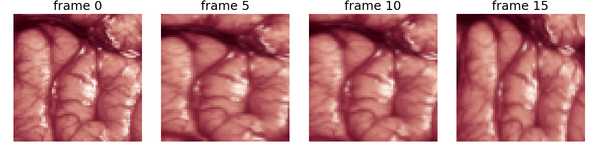
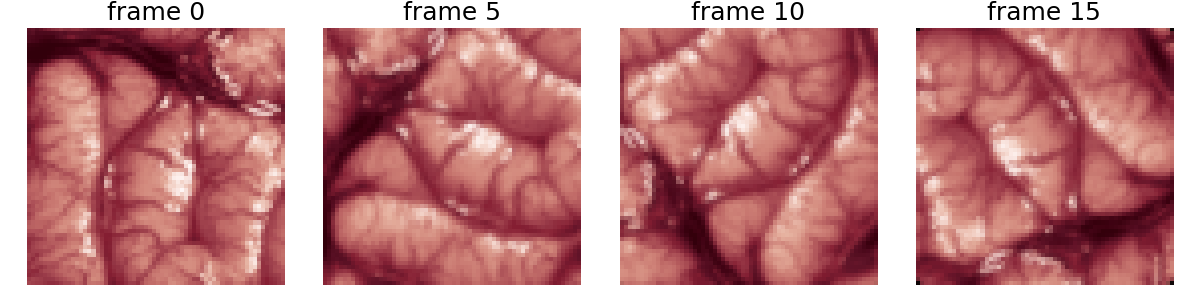
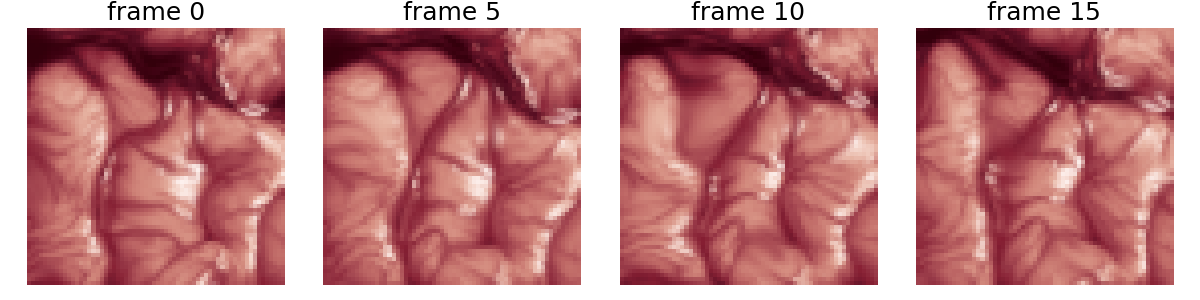
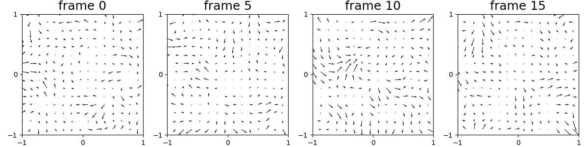
Random elastic deformation
Elastic deformation creates a non-parametric motion that can simulate tissue deformation or fluid motion.
- Parameters:
magnitude_amp: Controls magnitude of deformations (in pixels)smoothness: Controls spatial correlation (higher = smoother)n_interpolation: Number of keyframes for temporal interpolation
magnitude_amp = 500  # Magnitude in pixels
smoothness = 5  # Spatial smoothness parameter
n_interpolation = 3  # Temporal interpolation points

def_field = ElasticDeformation(
    magnitude_amp,
    smoothness,
    img_shape,
    n_frames,
    n_interpolation,
    dtype=dtype,
    device=device,
)
elastic_std = def_field.compute_field_std()
print(
    f"Generated random elastic deformation field has an std of {elastic_std:.2f} pixels."
)
Generated random elastic deformation field has an std of 5.77 pixels.
x_motion = def_field(x, 0, n_frames, mode=simu_interp)
x_motion = x_motion.moveaxis(time_dim, 1)
print("x_motion.shape:", x_motion.shape)
x_motion.shape: torch.Size([1, 50, 3, 88, 88])
n_frames_display = 5

if thumbnail:
    # plot few frames as thumbnails
    n_rows, n_cols = 1, 4
    plt.figure(figsize=(12, 3))
    for frame in range(n_frames):
        n_frame = n_frames_display * frame
        if n_frame >= n_frames or frame >= n_rows * n_cols:
            break
        plt.subplot(n_rows, n_cols, frame + 1)
        x_frame = (
            x_motion[0, n_frame, :, amp_max : n + amp_max, amp_max : n + amp_max]
            .moveaxis(0, -1)
            .view(*fov_shape, n_wav)
            .cpu()
            .numpy()
        )
        plt.imshow(x_frame, cmap="gray")  # in X
        plt.title("frame %d" % (n_frame), fontsize=18)
        plt.axis("off")
    plt.tight_layout()
    plt.show()
else:
    # show motion as video with IPython display
    from IPython.display import clear_output

    x_min, x_max = x_motion.min().item(), x_motion.max().item()
    for frame in range(n_frames):
        n_frame = n_frames_display * frame
        if n_frame >= n_frames:
            break
        plt.close()
        x_frame = (
            x_motion[0, n_frame, :, amp_max : n + amp_max, amp_max : n + amp_max]
            .moveaxis(0, -1)
            .view(*fov_shape, n_wav)
            .cpu()
            .numpy()
        )
        plt.imshow(x_frame, cmap="gray", vmin=x_min, vmax=x_max)  # in X
        plt.suptitle("frame %d" % (n_frame), fontsize=16)
        plt.colorbar(fraction=0.046, pad=0.04)
        plt.pause(0.01)
        clear_output(wait=True)
interval = torch.linspace(0, img_size - 1, img_size, dtype=torch.float64)
x1, x2 = torch.meshgrid(interval, interval, indexing="xy")

x1, x2 = x1 / img_size * 2 - 1, x2 / img_size * 2 - 1

x1, x2 = x1.cpu().numpy(), x2.cpu().numpy()
field = def_field.field.cpu().numpy()

n_frames_display = 5

if thumbnail:
    # plot few frames
    plt.figure(figsize=(12, 3))
    n_rows, n_cols = 1, 4
    for frame in range(n_frames):
        n_frame = n_frames_display * frame
        if n_frame >= n_frames or frame >= n_rows * n_cols:
            break
        plt.subplot(n_rows, n_cols, frame + 1)
        step = 6  # change this to plot fewer or more arrows
        plt.quiver(
            x1[::step, ::step],
            -x2[::step, ::step],
            (field[n_frame, ::step, ::step, 0] - x1[::step, ::step]),
            -(field[n_frame, ::step, ::step, 1] - x2[::step, ::step]),
            angles="xy",
            scale_units="xy",
            scale=1,
        )
        plt.title("frame %d" % (n_frame), fontsize=18)
        # Make axes square so quiver arrows reflect image aspect ratio
        ax = plt.gca()
        ax.set_aspect("equal", adjustable="box")
        ax.set_xlim([-1, 1])
        ax.set_ylim([-1, 1])
        ax.set_xticks([-1, 0, 1])
        ax.set_yticks([-1, 0, 1])
    plt.tight_layout()
    plt.show()
else:
    # show motion as video with IPython display
    from IPython.display import clear_output

    for frame in range(n_frames):
        n_frame = n_frames_display * frame
        if n_frame >= n_frames:
            break
        plt.figure(figsize=(6, 6))
        step = 6  # change this to plot fewer or more arrows
        plt.quiver(
            x1[::step, ::step],
            -x2[::step, ::step],
            (field[n_frame, ::step, ::step, 0] - x1[::step, ::step]),
            -(field[n_frame, ::step, ::step, 1] - x2[::step, ::step]),
            angles="xy",
            scale_units="xy",
            scale=1,
        )
        plt.suptitle("frame %d" % n_frame, fontsize=16)
        # Make axes square so quiver arrows reflect image aspect ratio
        plt.pause(0.01)
        clear_output(wait=True)
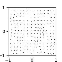
Plot a frame of the deformation field for thumbnail sphinx_gallery_thumbnail_number = 7
n_frame = 30
plt.figure(figsize=(2, 2))
step = 6  # change this to plot fewer or more arrows
plt.quiver(
    x1[::step, ::step],
    -x2[::step, ::step],
    (field[n_frame, ::step, ::step, 0] - x1[::step, ::step]),
    -(field[n_frame, ::step, ::step, 1] - x2[::step, ::step]),
    angles="xy",
    scale_units="xy",
    scale=1,
)
# Make axes square so quiver arrows reflect image aspect ratio
ax = plt.gca()
ax.set_aspect("equal", adjustable="box")
ax.set_xlim([-1, 1])
ax.set_ylim([-1, 1])
ax.set_xticks([-1, 0, 1])
ax.set_yticks([-1, 0, 1])
plt.show()
Total running time of the script: (0 minutes 2.554 seconds)