06.b. Dynamic acquisitions + reconstruction

This tutorial shows how to simulate measurements of dynamic scenes using the spyrit.core.meas submodule. It also demonstrates how to reconstruct a clean image of the scene through motion compensation.

It is based on the spyrit.core.meas.DynamicHadamSplit2d class of the spyrit.core.meas submodule.

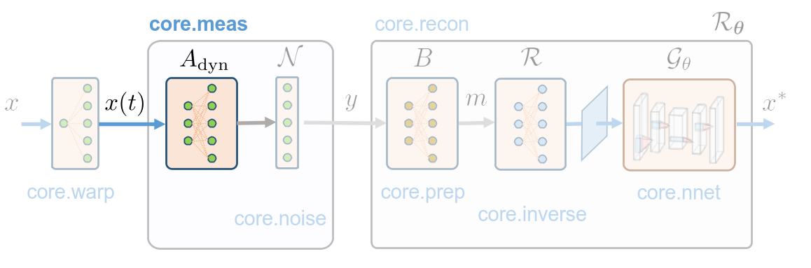
We consider the inverse problem

\[y = \text{diag}(A x_{t=1,..., 2M}),\]

where \(A \colon\, \mathbb{R}_+^{2M\times N}\) is the acquisition matrix that contains positive DMD patterns, \(x_{t=1,..., 2M} \in \mathbb{R}^{N \times 2M}\) is the temporal signal of interest, \(2M\) is both the number of DMD patterns (positives and negatives) and the number of frames, \(N\) is the dimension of the signal within the field of view, \(\text{diag}\colon\, \mathbb{R}^{2M \times 2M} \to \mathbb{R}^{2M}\) extracts the diagonal of its input.

Dynamic single-pixel imaging aims to reconstruct the temporal sequence \(x_{t=1,..., 2M}\). Our approach is based on motion-compensation. Assuming known motion during the acquisition, we build a new forward operator \(A_{\rm dyn}\) that compensates the motion to a static reference frame \(x\), i.e. such that

\[\text{diag}(A x_{t=1,..., 2M}) = A_{\rm dyn} x.\]

Important

The theory behind dynamic single-pixel imaging with motion compensation is detailed in [Maitre2024_1], [Maitre2024_2], [Maitre2026].

Warning

This tutorial assumes the reader is already familiar with the static measurements operators. If not, we recommend starting with the tutorials 1a, 1b, and 1c.

Key concepts:

• Simulation of a dynamic single-pixel acquisition accounting for motion during the measurement process

• Creation of a dynamic forward operator \(A_{\text{dyn}}\) using motion compensation with pattern warping or image warping

• Numerical evidence that image warping is better suited for unbiased simulations

• Regularized reconstruction with finite differences

import torch
import torchvision
import matplotlib.pyplot as plt
import os
import math
import time

from pathlib import Path

from spyrit.misc.disp import torch2numpy
from spyrit.misc.statistics import transform_norm
import spyrit.misc.metrics as score
from spyrit.misc.load_data import download_girder

import spyrit.core.torch as spytorch
from spyrit.core.prep import Unsplit
from spyrit.core.warp import AffineDeformationField

Set acquisition parameters:

• img_size: Full image resolution (pixels)

• n: Measurement pattern size (defines FOV)

• und: Undersampling factor (1 = no undersampling)

• M: Total number of measurements per frame

img_size = 88  # Full image side's size in pixels
n = 64  # Measurement pattern side's size in pixels (Field of View)
und = 1  # Undersampling factor (1 = full sampling)

M = n**2 // und  # Number of (positive, negative) measurements

print(f"Image size: {img_size}x{img_size}")
print(f"Measurement FOV: {n}x{n}")
print(f"Measurements: {M}")

# Dataset parameters
i = 0  # Image index (modify to change the image)
spyritPath = "../data/data_online/"
imgs_path = os.path.join(spyritPath, "spyrit/")

# Computation parameters
device = torch.device("cuda" if torch.cuda.is_available() else "cpu")
print(f"Using device: {device}")

dtype = (
    torch.float32
)  # Low precision for tutorial stability, feel free to use torch.float64 for better accuracy if memory allows
simu_interp = "bilinear"  # Interpolation for motion simulation
reco_interp = "bilinear"  # Interpolation for building forward operator

time_dim = 1  # Time dimension index in tensors

# Derived parameters
meas_shape = (n, n)
img_shape = (img_size, img_size)
amp_max = (img_shape[0] - meas_shape[0]) // 2  # Border size for centering FOV

Image size: 88x88
Measurement FOV: 64x64
Measurements: 4096
Using device: cpu

Load an image from Tomoradio’s warehouse.

# Download an RGB brain surface image.
url_tomoradio = "https://tomoradio-warehouse.creatis.insa-lyon.fr/api/v1"
data_root = Path("../data/data_online/2025_dynamic")  # local path to data
imgs_path = data_root / Path("images/")
id_files = [
    "69248e3204d23f6e964b16b7",  # brain_surface_colorized.png
]
try:
    download_girder(url_tomoradio, id_files, imgs_path)
except Exception as e:
    print("Unable to download from the Tomoradio warehouse")
    print(e)

# Create a transform for natural images to normalized image tensors
transform = transform_norm(img_size=img_size)
batch_size = 1

# Create dataset and loader
dataset = torchvision.datasets.ImageFolder(root=data_root, transform=transform)
dataloader = torch.utils.data.DataLoader(dataset, batch_size=batch_size)

img, _ = dataloader.dataset[0]
x = img.unsqueeze(0).to(dtype=dtype, device=device)

print(f"Shape of input images: {x.shape}")

x = (x - x.min()) / (x.max() - x.min())
n_wav = x.shape[1]

File already exists at ../data/data_online/2025_dynamic/images/brain_surface_colorized.png
Shape of input images: torch.Size([1, 3, 88, 88])

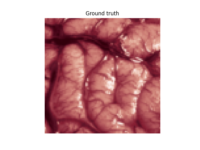
Plot the reference image

x_plot = x.moveaxis(1, -1).squeeze().cpu().numpy()

plt.imshow(x_plot)
if n_wav == 1:
    plt.colorbar(fraction=0.046, pad=0.04)
plt.title("Ground truth")
plt.axis("off")
plt.show()

Define motion model and deformation fields

We simulate a pulsating motion using affine transformations (see tutorial 6a).

Both forward and inverse deformation fields are needed for the tutorial:

• Forward field: for motion simulation & reconstruction with image warping

• Inverse field: for reconstruction with pattern warping

a = 0.2  # Scaling amplitude
T = 1000  # Period of motion cycle

print(f"Motion parameters:")
print(f"  Amplitude: {a:.2f}")
print(f"  Period: {T} ms")


def s(t):
    return 1 + a * math.sin(t * 2 * math.pi / T)


def f(t):
    return torch.tensor(
        [
            [1 / s(t), 0, 0],
            [0, s(t), 0],
            [0, 0, 1],
        ],
        dtype=dtype,
    )


def f_inv(t):
    return torch.tensor(
        [
            [s(t), 0, 0],
            [0, 1 / s(t), 0],
            [0, 0, 1],
        ],
        dtype=dtype,
    )


# Create time vector for 2*M frames (positive + negative measurements)
n_frames = 2 * M
time_vector = torch.linspace(0, 2 * T, n_frames)
print(f"Time vector: {n_frames} frames from 0 to {2*T}ms")

# Create instances of affine deformation fields
def_field = AffineDeformationField(
    f, time_vector, img_shape, dtype=dtype, device=device
)
def_field_inv = AffineDeformationField(
    f_inv, time_vector, img_shape, dtype=dtype, device=device
)

print(f"Created deformation fields with shape: {def_field.field.shape}")

Motion parameters:
  Amplitude: 0.20
  Period: 1000 ms
Time vector: 8192 frames from 0 to 2000ms
Created deformation fields with shape: torch.Size([8192, 88, 88, 2])

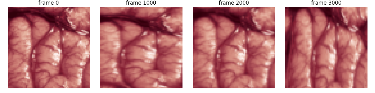
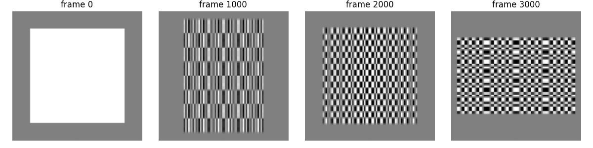
We apply the deformation field to create a dynamic image sequence

x_motion = def_field(x, 0, n_frames, mode=simu_interp)
x_motion = x_motion.moveaxis(time_dim, 1)
print(f"Dynamic sequence shape: {x_motion.shape}")
print(f"Generated {x_motion.shape[1]} frames for acquisition simulation")

Dynamic sequence shape: torch.Size([1, 8192, 3, 88, 88])
Generated 8192 frames for acquisition simulation

We display a few frames to visualize the motion.

# plot few frames
n_frames_display = 1000

plt.figure(figsize=(12, 3))
n_rows, n_cols = 1, 4
for frame in range(n_frames):
    n_frame = n_frames_display * frame
    if n_frame >= n_frames or frame >= n_rows * n_cols:
        break
    plt.subplot(n_rows, n_cols, frame + 1)
    plt.imshow(
        x_motion[
            0, n_frame, :, amp_max : img_size - amp_max, amp_max : img_size - amp_max
        ]
        .moveaxis(0, -1)
        .view(*meas_shape, n_wav)
        .cpu()
        .numpy(),
        cmap="gray",
    )  # in X
    plt.title("frame %d" % (n_frame), fontsize=12)
    plt.axis("off")
plt.tight_layout()
plt.show()

Dynamic measurement simulation

We simulate a dynamic single-pixel acquisition.

Note

The dynamic measurement operator classes extend the static ones:

• Linear -> DynamicLinear

• LinearSplit -> DynamicLinearSplit

• HadamSplit2d -> DynamicHadamSplit2d

We used the DynamicHadamSplit2d class (specialized for Hadamard patterns) for this tutorial.

from spyrit.core.meas import DynamicHadamSplit2d

meas_op = DynamicHadamSplit2d(
    time_dim=time_dim,
    h=n,
    M=M,
    order=None,
    fast=True,
    reshape_output=False,
    img_shape=img_shape,
    noise_model=torch.nn.Identity(),
    white_acq=None,
    dtype=dtype,
    device=device,
)

t1 = time.time()
y1 = meas_op(x_motion)
t2 = time.time()

print(f"Computation time: {t2 - t1:.3f}s")
print(f"Output shape: {y1.shape}")

Computation time: 0.601s
Output shape: torch.Size([1, 3, 8192])

We preprocess measurements for reconstruction using the differential strategy to combine the positive/negative measurements.

prep_op = Unsplit()
y2 = prep_op(y1)

print(f"\nMeasurement processing:")
print(f"  Raw measurements shape: {y1.shape}")
print(f"  Processed measurements shape: {y2.shape}")

Measurement processing:
  Raw measurements shape: torch.Size([1, 3, 8192])
  Processed measurements shape: torch.Size([1, 3, 4096])

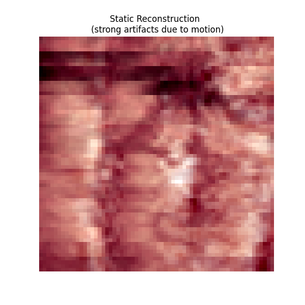
Static reconstruction baseline

Compute a static reconstruction for comparison. This ignores motion and treats all measurements as from a static scene.

from spyrit.core.meas import HadamSplit2d

meas_op_stat = HadamSplit2d(h=n, M=M, order=None, dtype=dtype, device=device)

print(f"\n=== Static Reconstruction (Baseline) ===")
x_stat = meas_op_stat.fast_pinv(y2)
print(f"Static reconstruction shape: {x_stat.shape}")

# Quick quality check for static reconstruction
x_ref_fov = x[0, :, amp_max : n + amp_max, amp_max : n + amp_max]
static_psnr = score.psnr(torch2numpy(x_stat), torch2numpy(x_ref_fov))
print(f"Static reconstruction PSNR: {static_psnr:.2f} dB")

plt.figure(figsize=(6, 6))
plt.imshow(torch2numpy(x_stat.moveaxis(1, -1).squeeze()))
plt.title("Static Reconstruction \n (strong artifacts due to motion)")
plt.axis("off")
plt.show()

=== Static Reconstruction (Baseline) ===
Static reconstruction shape: torch.Size([1, 3, 64, 64])
Static reconstruction PSNR: 19.86 dB
Clipping input data to the valid range for imshow with RGB data ([0..1] for floats or [0..255] for integers). Got range [-0.21864055..1.0663859].

We set up regularization for the inverse problem with first-order finite differences (smoothing prior). We use Neumann boundary conditions.

Dx, Dy = spytorch.neumann_boundary(img_shape)
D2 = Dx.T @ Dx + Dy.T @ Dy
D2 = D2.to(dtype=dtype)

print(f"Regularization matrix shape: {D2.shape}")

Regularization matrix shape: torch.Size([7744, 7744])

Build dynamic system matrix

Construct the dynamic forward operator \(H_{\rm dyn}\) that accounts for motion. This matrix maps the reference image to measurements accounting for motion.

Two approaches:

1. warping='pattern': Warp the patterns. Need to pass the inverse deformation field.

2. warping='image': Warp the image. Need to pass the forward deformation field.

1. Pattern warping

# Build the dynamic system matrix
print("Building H_dyn using pattern warping (inverse deformation)...")
meas_op.build_dynamic_forward(
    def_field_inv, warping="pattern", mode=reco_interp, verbose=False
)

print(f"Dynamic system matrix shape: {meas_op.A_dyn.shape}")
print(
    f"Dynamic system matrix (differential strategy AFTER motion compensation) shape: {meas_op.H_dyn.shape}"
)

Building H_dyn using pattern warping (inverse deformation)...
Be careful to use the inverse deformation field when warping patterns.
Dynamic system matrix shape: torch.Size([8192, 7744])
Dynamic system matrix (differential strategy AFTER motion compensation) shape: torch.Size([4096, 7744])

Note

In order to use the differential strategy with dynamic scenes, it is important to build the dynamic system matrix after motion compensation [Maitre2026].

Verify forward model accuracy

Test the dynamic forward model by computing the residual of the forward model. Without measurement noise and using dtype=float64, the residual should be very small (\(\approx\) 1e-12) [Maitre2024_2]. When using the pattern warping approach, the forward model is non-zero, indicating a bias in the model.

A_dyn_x = meas_op.forward_A_dyn(x)
residual_norm = torch.norm(y1 - A_dyn_x).item()
relative_error = residual_norm / torch.norm(y1).item()

print(f"\n=== Forward Model Verification ===")
print(f"  Predicted measurements shape: {A_dyn_x.shape}")
print(f"  Residual norm: {residual_norm:.2e}")
print(f"  Relative error: {relative_error:.2e}")

# Visualize residual pattern (averaged over spectral channels)
plt.figure(figsize=(4, 6))
residual_2d = abs(y1 - A_dyn_x).mean(dim=1).squeeze().cpu().numpy().reshape((2 * n, n))
plt.imshow(residual_2d, cmap="Spectral")
plt.colorbar(fraction=0.046 * 6 / 3, pad=0.04)
plt.title(f"Forward Model Residual |y - A_dyn·x| \n Max: {residual_2d.max():.2e}")
plt.tight_layout()
plt.show()

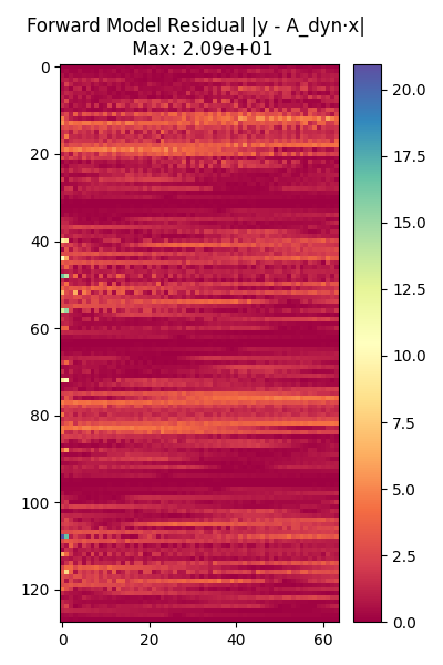
=== Forward Model Verification ===
  Predicted measurements shape: torch.Size([1, 3, 8192])
  Residual norm: 2.84e+02
  Relative error: 1.78e-03

We display few dynamic patterns.

print(f"\nVisualizing dynamic matrix evolution...")
H_dyn_diff_np = torch2numpy(meas_op.H_dyn)

# plot few patterns
n_frames_display = 500

plt.figure(figsize=(12, 3))
n_rows, n_cols = 1, 4
for frame in range(n_frames):
    n_frame = n_frames_display * frame
    if n_frame >= n_frames or frame >= n_rows * n_cols:
        break
    plt.subplot(n_rows, n_cols, frame + 1)
    plt.imshow(
        H_dyn_diff_np[n_frame].reshape(img_shape), cmap="gray", vmin=-1, vmax=1
    )  # in X_{ext}
    plt.title("frame %d" % (2 * n_frame), fontsize=12)
    plt.axis("off")
plt.tight_layout()
plt.show()

Visualizing dynamic matrix evolution...

Analyze system conditioning

Move computations to CPU for optimized linear algebra.

print(f"\n=== Preparing for Reconstruction ===")
print("Moving to CPU for optimized linear algebra...")
H_dyn = meas_op.H_dyn.cpu()
y2 = y2.cpu()

=== Preparing for Reconstruction ===
Moving to CPU for optimized linear algebra...

Compute singular values to understand the inverse problem difficulty. High condition number indicates need for regularization.

print("Analyzing system matrix conditioning...")
sing_vals = torch.linalg.svdvals(H_dyn)
condition_number = (sing_vals[0] / sing_vals[-1]).item()
sigma_max = sing_vals[0].item()
sigma_min = sing_vals[-1].item()

print(f"Singular value spectrum:")
print(f"  Maximum: {sigma_max:.2e}")
print(f"  Minimum: {sigma_min:.2e}")
print(f"  Condition number: {condition_number:.2e}")

Analyzing system matrix conditioning...
Singular value spectrum:
  Maximum: 1.11e+02
  Minimum: 9.78e-02
  Condition number: 1.13e+03

Solve the regularized least squares problem

\[\arg \min_x \frac{1}{2} \| y - H_{\rm dyn}^{\rm wp} x \|^2 + \frac{\tilde{\eta}}{2} \| D x \|^2\]

where \(\tilde{\eta}\) is the normalized regularization parameter scaled by the maximum singular value of \(H_{\rm dyn}\) and \(D\) is a first order finite difference operator.

eta = 1e-5  # Regularization parameter (adjust based on noise level)

print(f"\n=== Dynamic Reconstruction ===")
print(f"Regularization parameter: {eta:.1e}")

start_time = time.time()
x_dyn_wp = torch.linalg.solve(
    H_dyn.T @ H_dyn + eta * sigma_max**2 * D2, H_dyn.T @ y2.moveaxis(1, -1)
)
solve_time = time.time() - start_time

print(f"Reconstruction completed in {solve_time:.2f}s")
print(f"Solution shape: {x_dyn_wp.shape}")

=== Dynamic Reconstruction ===
Regularization parameter: 1.0e-05
Reconstruction completed in 9.33s
Solution shape: torch.Size([1, 7744, 3])

We plot the dynamic reconstruction

x_dyn_wp_plot = x_dyn_wp.view(*img_shape, n_wav)

plt.figure(figsize=(6, 6))
plt.imshow(x_dyn_wp_plot.cpu().numpy(), cmap="gray")
plt.title(
    "Dynamic Reconstruction \n (Motion Compensated with pattern warping)", fontsize=14
)
plt.axis("off")
if n_wav == 1:
    plt.colorbar(fraction=0.046, pad=0.04)

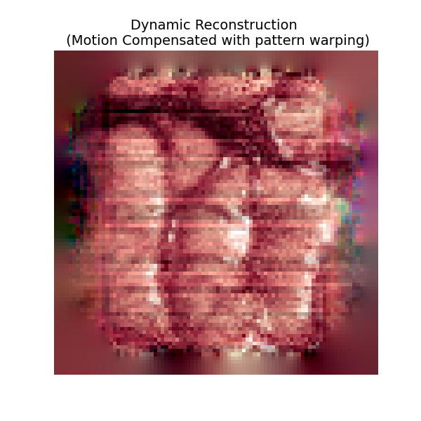
Clipping input data to the valid range for imshow with RGB data ([0..1] for floats or [0..255] for integers). Got range [-0.39748687..1.2340564].

2. Image warping

# Build the dynamic system matrix
print("Building H_dyn using image warping (forward deformation)...")
meas_op.build_dynamic_forward(
    def_field, warping="image", mode=reco_interp, verbose=False
)

print(
    f"Dynamic system matrix (differential strategy AFTER motion compensation) shape: {meas_op.H_dyn.shape}"
)

Building H_dyn using image warping (forward deformation)...
Dynamic system matrix (differential strategy AFTER motion compensation) shape: torch.Size([4096, 7744])

Verify forward model accuracy

Test the dynamic forward model by computing the residual of the forward model. Without measurement noise and using dtype=float64, the residual should be very small (\(\approx\) 1e-12) [Maitre2024_2]. When using the image warping approach, the forward model is almost zero, indicating no bias in the model.

A_dyn_x = meas_op.forward_A_dyn(x)
residual_norm = torch.norm(y1 - A_dyn_x).item()
relative_error = residual_norm / torch.norm(y1).item()

print(f"\n=== Forward Model Verification ===")
print(f"  Predicted measurements shape: {A_dyn_x.shape}")
print(f"  Residual norm: {residual_norm:.2e}")
print(f"  Relative error: {relative_error:.2e}")

# Visualize residual pattern (averaged over spectral channels)
plt.figure(figsize=(4, 6))
residual_2d = abs(y1 - A_dyn_x).mean(dim=1).squeeze().cpu().numpy().reshape((2 * n, n))
plt.imshow(residual_2d, cmap="Spectral")
plt.colorbar(fraction=0.046 * 6 / 3, pad=0.04)
plt.title(f"Forward Model Residual |y - A_dyn·x| \n Max: {residual_2d.max():.2e}")
plt.tight_layout()
plt.show()

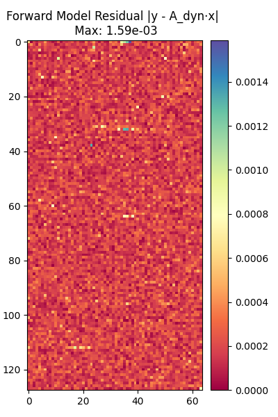
=== Forward Model Verification ===
  Predicted measurements shape: torch.Size([1, 3, 8192])
  Residual norm: 4.04e-02
  Relative error: 2.53e-07

We display few dynamic patterns

print(f"\nVisualizing dynamic matrix evolution...")
H_dyn_diff_np = torch2numpy(meas_op.H_dyn)

# plot few patterns
n_frames_display = 500

plt.figure(figsize=(12, 3))
n_rows, n_cols = 1, 4
for frame in range(n_frames):
    n_frame = n_frames_display * frame
    if n_frame >= n_frames or frame >= n_rows * n_cols:
        break
    plt.subplot(n_rows, n_cols, frame + 1)
    plt.imshow(
        H_dyn_diff_np[n_frame].reshape(img_shape), cmap="gray", vmin=-1, vmax=1
    )  # in X_{ext}
    plt.title("frame %d" % (2 * n_frame), fontsize=12)
    plt.axis("off")
plt.tight_layout()
plt.show()

Visualizing dynamic matrix evolution...

Analyze system conditioning

Move computations to CPU for optimized linear algebra.

print(f"\n=== Preparing for Reconstruction ===")
print("Moving to CPU for optimized linear algebra...")
H_dyn = meas_op.H_dyn.cpu()
y2 = y2.cpu()

=== Preparing for Reconstruction ===
Moving to CPU for optimized linear algebra...

Compute singular values to understand the inverse problem difficulty. High condition number indicates need for regularization.

print("Analyzing system matrix conditioning...")
sing_vals = torch.linalg.svdvals(H_dyn)
condition_number = (sing_vals[0] / sing_vals[-1]).item()
sigma_max = sing_vals[0].item()
sigma_min = sing_vals[-1].item()

print(f"Singular value spectrum:")
print(f"  Maximum: {sigma_max:.2e}")
print(f"  Minimum: {sigma_min:.2e}")
print(f"  Condition number: {condition_number:.2e}")

Analyzing system matrix conditioning...
Singular value spectrum:
  Maximum: 1.10e+02
  Minimum: 2.39e-01
  Condition number: 4.61e+02

Solve the regularized least squares problem

\[\arg \min_x \frac{1}{2} \| y - H_{\rm dyn}^{\rm wf} x \|^2 + \frac{\tilde{\eta}}{2} \| D x \|^2\]

where \(\tilde{\eta}\) is the normalized regularization parameter scaled by the maximum singular value of \(H_{\rm dyn}\) and \(D\) is a first order finite difference operator.

eta = 1e-5  # Regularization parameter (adjust based on noise level)

print(f"\n=== Dynamic Reconstruction ===")
print(f"Regularization parameter: {eta:.1e}")

start_time = time.time()
x_dyn_wf = torch.linalg.solve(
    H_dyn.T @ H_dyn + eta * sigma_max**2 * D2, H_dyn.T @ y2.moveaxis(1, -1)
)
solve_time = time.time() - start_time

print(f"Reconstruction completed in {solve_time:.2f}s")
print(f"Solution shape: {x_dyn_wf.shape}")

=== Dynamic Reconstruction ===
Regularization parameter: 1.0e-05
Reconstruction completed in 9.38s
Solution shape: torch.Size([1, 7744, 3])

We plot the dynamic reconstruction

x_dyn_wf_plot = x_dyn_wf.view(*img_shape, n_wav)

plt.figure(figsize=(6, 6))
plt.imshow(x_dyn_wf_plot.cpu().numpy(), cmap="gray")
plt.title(
    "Dynamic Reconstruction \n (Motion Compensated with image warping)", fontsize=14
)
plt.axis("off")
if n_wav == 1:
    plt.colorbar(fraction=0.046, pad=0.04)

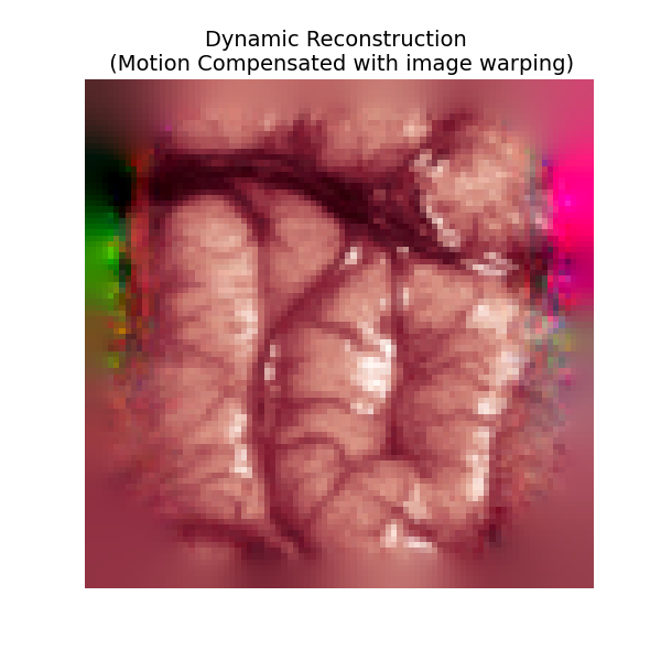
Clipping input data to the valid range for imshow with RGB data ([0..1] for floats or [0..255] for integers). Got range [-0.5651888..1.5256104].

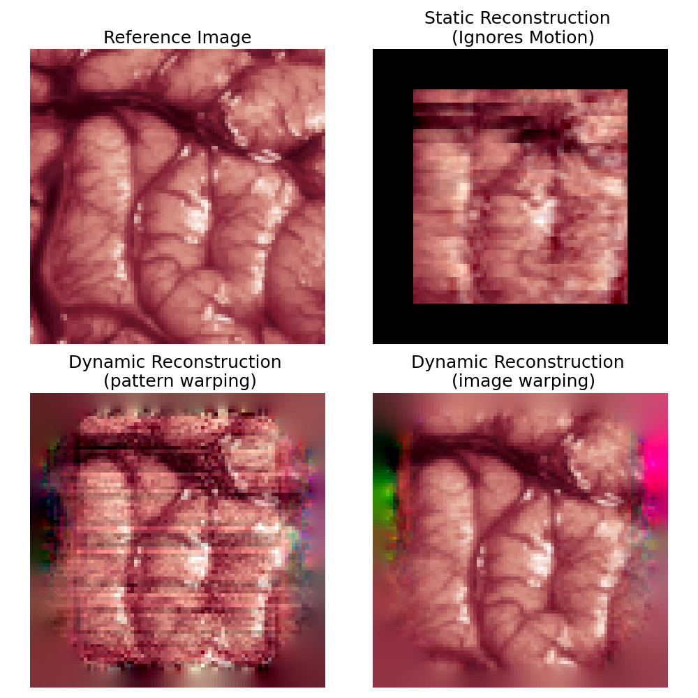
Results overview

Compare the original image, static reconstruction, and dynamic reconstruction. This shows the improvement gained by accounting for motion.

sphinx_gallery_thumbnail_number = 10

print(f"\n=== Reconstruction Comparison ===")
fig, ax = plt.subplots(2, 2, figsize=(10, 10))

# Original reference image
ref_img = x.view(n_wav, *img_shape).moveaxis(0, -1).cpu().numpy()

im0 = ax[0, 0].imshow(ref_img, cmap="gray")
ax[0, 0].set_title("Reference Image", fontsize=18)
ax[0, 0].axis("off")
if n_wav == 1:
    fig.colorbar(im0, ax=ax[0, 0], fraction=0.046, pad=0.04)

# Static reconstruction
static_img = torch.zeros((*img_shape, n_wav), dtype=dtype, device=device)
static_img[amp_max : n + amp_max, amp_max : n + amp_max] = x_stat.view(
    n_wav, *meas_shape
).moveaxis(0, -1)

im1 = ax[0, 1].imshow(static_img.cpu().numpy(), cmap="gray")
ax[0, 1].set_title("Static Reconstruction \n (Ignores Motion)", fontsize=18)
ax[0, 1].axis("off")
if n_wav == 1:
    fig.colorbar(im1, ax=ax[0, 1], fraction=0.046, pad=0.04)

# Dynamic reconstruction with pattern warping
im2 = ax[1, 0].imshow(x_dyn_wp_plot.cpu().numpy(), cmap="gray")
ax[1, 0].set_title("Dynamic Reconstruction \n (pattern warping)", fontsize=18)
ax[1, 0].axis("off")
if n_wav == 1:
    fig.colorbar(im2, ax=ax[1, 0], fraction=0.046, pad=0.04)

# Dynamic reconstruction with image warping
im3 = ax[1, 1].imshow(x_dyn_wf_plot.cpu().numpy(), cmap="gray")
ax[1, 1].set_title("Dynamic Reconstruction \n (image warping)", fontsize=18)
ax[1, 1].axis("off")
if n_wav == 1:
    fig.colorbar(im3, ax=ax[1, 1], fraction=0.046, pad=0.04)

plt.tight_layout()
plt.show()

=== Reconstruction Comparison ===
Clipping input data to the valid range for imshow with RGB data ([0..1] for floats or [0..255] for integers). Got range [-0.21864055..1.0663859].
Clipping input data to the valid range for imshow with RGB data ([0..1] for floats or [0..255] for integers). Got range [-0.39748687..1.2340564].
Clipping input data to the valid range for imshow with RGB data ([0..1] for floats or [0..255] for integers). Got range [-0.5651888..1.5256104].

Compute image quality metrics to quantify reconstruction improvement. Metrics are computed in the FOV region for fair comparison.

# Extract FOV region for metric calculation
x_dyn_wp_in_X = x_dyn_wp_plot[amp_max : n + amp_max, amp_max : n + amp_max]
x_dyn_wf_in_X = x_dyn_wf_plot[amp_max : n + amp_max, amp_max : n + amp_max]

x_ref_in_X = x[0, :, amp_max : n + amp_max, amp_max : n + amp_max].moveaxis(0, -1)

# Calculate metrics for both reconstructions
psnr_static = score.psnr(
    torch2numpy(x_stat.view(n_wav, *meas_shape).moveaxis(0, -1)),
    torch2numpy(x_ref_in_X),
)
ssim_static = score.ssim(
    torch2numpy(x_stat.view(n_wav, *meas_shape).moveaxis(0, -1)),
    torch2numpy(x_ref_in_X),
)

psnr_dynamic_wp = score.psnr(torch2numpy(x_dyn_wp_in_X), torch2numpy(x_ref_in_X))
ssim_dynamic_wp = score.ssim(torch2numpy(x_dyn_wp_in_X), torch2numpy(x_ref_in_X))

psnr_dynamic_wf = score.psnr(torch2numpy(x_dyn_wf_in_X), torch2numpy(x_ref_in_X))
ssim_dynamic_wf = score.ssim(torch2numpy(x_dyn_wf_in_X), torch2numpy(x_ref_in_X))

print(f"\n=== Quantitative Results (in the SPC FOV X) ===")
print(f"{'Method':<25} {'PSNR (dB)':<12} {'SSIM'}")
print("-" * 48)
print(f"{'Static':<25} {psnr_static:<12.2f} {ssim_static:.3f}")
print(
    f"{'Dynamic (pattern warping)':<25} {psnr_dynamic_wp:<12.2f} {ssim_dynamic_wp:.3f}"
)
print(f"{'Dynamic (image warping)':<25} {psnr_dynamic_wf:<12.2f} {ssim_dynamic_wf:.3f}")
print("-" * 48 + "\n")

improvement_wp = psnr_dynamic_wp - psnr_static
improvement_wf = psnr_dynamic_wf - psnr_static

print(
    f"Dynamic reconstruction (pattern warping) achieved a PSNR improvement of {improvement_wp:.2f} dB over static reconstruction."
)
print(
    f"Dynamic reconstruction (image warping) achieved a PSNR improvement of {improvement_wf:.2f} dB over static reconstruction."
)

=== Quantitative Results (in the SPC FOV X) ===
Method                    PSNR (dB)    SSIM
------------------------------------------------
Static                    19.86        0.835
Dynamic (pattern warping) 25.16        0.943
Dynamic (image warping)   34.30        0.996
------------------------------------------------

Dynamic reconstruction (pattern warping) achieved a PSNR improvement of 5.30 dB over static reconstruction.
Dynamic reconstruction (image warping) achieved a PSNR improvement of 14.44 dB over static reconstruction.